Transformers for Vision

Vision Transformers

Vision transformers are quickly becoming popular in the space of computer vision. Where convolution neural networks (CNNs) once reigned supreme, vision transformers are quickly giving CNNs a run for their money. A quick look at paperswithcode SOTA for imagenet image classification shows that 4 out of the top 5 models incorporate some form of a transformer.

A step-by-step walkthrough

To understand transformers for vision, it helps to have a working understanding of the original Attention is all you Need Paper and ideally a little about CNNs. In this walkthrough, I’ll go through the paper An Image is Worth 16x16 Words: Transformers for Image Recognition at Scale. For a full copy of the notebook, click here. The code here will be simplified for educational purposes.

Embeddings

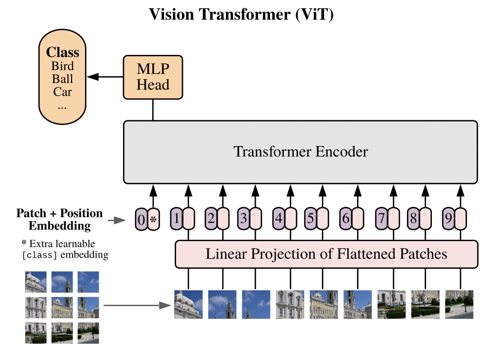
Transformers for vision work almost identical to a standard transformer. Vision transformers split an image into smaller patches, where each patch is passed into the transfomer as a token. In the paper, they used 16x16 patches. Here patches refers to the number of patches that make up an image, not the number of pixels per patch. For example, Imagenet pictures are 224 x 224 pixels, so when we want our image to be split up into 16x16 patches, we divide $\frac{224}{16}$ which tells us each patch is going to be made up of 14 x 14 pixels.

Since colored images are 3-dimensional (depth(R,G,B channels) x height x width), we need to use a convolution in order to generate a feature map which can act as our patches.

class PatchEmbeddings(nn.Module):
    def __init__(self, img_size, patch_size, embed_dim, input_channels):
        super().__init__()
        self.img_size = img_size
        self.patch_size = patch_size
        assert img_size % patch_size == 0
        self.num_patches = (img_size // patch_size) ** 2
        
        # we use convolution to create the projections of input image(3d matrix) to a vector
        # each filter is responsible for creating one patch 
        self.proj = nn.Conv2d(
            in_channels = input_channels,
            out_channels = embed_dim,
            stride = patch_size,
            kernel_size = patch_size
        )

We then take an input tensor $x$ of shape (batch_size x input_channels x height x width). When then run our tensor through the convolution, which gives us a shape (batch_size x embed_dim x num_patches ** .5 x num_patches ** .5). We then flatten the tensor so that the last two dimensions so that our tensor has shape (batch_size x embed_dim x num_patches). We then swap the last two dimensions by transposing the matrix. We get an output tensor of shape (batch_size, num_patches, embed_dim).

    def forward(self, x):
        """
        converts a tensor of (batch_size x input_channels x height x width)
        to one of tensor of shape (batch_size, num_patches, embed_dim)
        """
        x = self.proj(x)
        x = x.flatten(2)
        x = x.transpose(-2, -1)
        return x
         

Note that this is only to get the patch embeddings. If we were to feed these embeddings into a transformer, it would have no sense of positional encodings, and each patch embedding would be treated as a bag of words.

Attention

Now that we have the patch embeddings done, the rest of the ViT is basically just a standard transformer. We first compute self-attention which is defined as softmax($\frac{QK^T}{\sqrt{d_k}})V$. In practice, we compute self-attention in batches, which is why we make use of torch.bmm for batch matrix multiplication.

def attention(query, key, value):
    """
    calculate scaled dot product attention given a q, k and v
    Params:
    query -> a given query tensor
    key -> a given key tensor
    value -> a given value tensor
    """
    dim = query.shape[-1]
    # (Query * tranpose(key)) / sqrt(dim)
    scores = torch.bmm(query, key.transpose(-2, -1)) / math.sqrt(dim)
    weights = F.softmax(scores, dim = -1)
    return torch.bmm(weights, value)

We generate the query, key, and value vectors by applying a separate learnable linear transformation to our input embedding $x$. To do this we make a separate class AttentionHead which will generate the separate Q, K, V vectors and compute the self-attention.

class AttentionHead(nn.Module):
    """
    Generates the Q, K, V vectors from a given input embedding x 
    and calculates the attention for one head
    Params:
    embed_dim -> embedding dimension of input vector x
    head_dim -> dimension that embed_dim gets transformed into from the qkv transformation
    """
    def __init__(self, embed_dim, head_dim):
        super().__init__()
        self.to_q = nn.Linear(embed_dim, head_dim)
        self.to_k = nn.Linear(embed_dim, head_dim)
        self.to_v = nn.Linear(embed_dim, head_dim)
    def forward(self, x):
        attn = attention(self.to_q(x), self.to_k(x), self.to_v(x))
        return attn

Now, we simply need to calculate multi-head attention. In multi-head attention, we downscale the dimensionality of each head proportional to the number of heads we have.

class MultiHeadAttention(nn.Module):
    """
    Calculates the Multi-Headed attention
    Params:
    num_heads -> number of heads to use, each head_dim is calculated as embed_dim // num_heads 
    embed_dim -> embedding dimension of vector x
    """
    def __init__(self, num_heads, embed_dim):
        super().__init__()
        self.embed_dim = embed_dim
        self.num_heads = num_heads
        self.head_dim = embed_dim // num_heads 

        self.heads = nn.ModuleList(
            AttentionHead(self.embed_dim, self.head_dim) 
            for _ in range(num_heads)
        )
        self.to_out = nn.Linear(embed_dim, embed_dim)

We then concatenate the outputs of each head together. We then take the concatenated matrix through a linear layer.

    def forward(self, x):
        # calculate attention for each head and concatenate tensor
        x = torch.cat([head(x) for head in self.heads], dim = -1)
        x = self.to_out(x)
        return x

MLP

The multi-layer perceptron is simply a feed forward neural network with an activation function between each linear layer.

class FeedForward(nn.Module):
    def __init__(self, embed_dim, hidden_dim, dropout = .1):
        """
        A feed forward network after scaled dot product attention
        Params:
        embed_dim = embedding dimension of vector
        hidden_dim = hidden dimension in the FF network, generally 2-4x larger than embed_dim
        dropout = % dropout for training
        """
        super().__init__()
        self.FFN = nn.Sequential(
            nn.Linear(embed_dim, hidden_dim),
            nn.GELU(),
            nn.Linear(hidden_dim, embed_dim),
            nn.Dropout(dropout)
        )
    def forward(self, x):
        x = self.FFN(x)
        return x

Dropout randomly zeroes out some elements from an input tensor with some probability $p$. This methods helps regularize the network which makes it more robust and avoid overfitting. Note that dropout only occurs during the training phase, when we validate the model, dropout is automatically set to 0. We also generally make the hidden dimension of the network 2-4x larger than the embedding dimension.

Putting the Encoder Together

class ViTBlock(nn.Module):
    """
    A full ViT encoder block, with a pre-layer normalization -> MHA -> layernorm ->FF
    Params:
    num_heads -> number of heads to use, each head_dim is calculated as embed_dim // num_heads
    embed_dim -> embedding dimension of vector x
    hidden_dim -> hidden dimension of the Feed Forward network, generally 2-4x larger than embed_dim
    """
    def __init__(self, num_heads, embed_dim, hidden_dim):
        super().__init__()
        self.MHA = MultiHeadAttention(num_heads, embed_dim)
        self.FFN = FeedForward(embed_dim, hidden_dim)

    def forward(self, x):
        x = self.MHA(x)
        x = self.FFN(x)
        return x

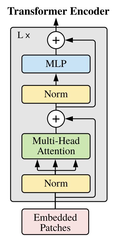
Great, we know have a working transformer encoder! Now all we need to do is stack as many encoders on top of each other and SOTA here we come!. Is it really that simple? Well it’s not that simple. If we just stack as many of these encoders on top of each other, we deal with the vanishing gradient problem. This happens during backpropagation when our activation functions (such as ReLU) will essentially “kill” neurons, which in turn gives us very small gradients which makes it impossible for our network to converge.

Luckily, we can solve this problem by adding residual connections. Residual connections help “smooth out” the loss landscape and help with the vanishing gradient problem. We can define a residual connection as $X^i = Layer_i(X) + X^{(i - 1)}$. Our output tensor $X$ after layer $i$ is equal to the output of $Layer_i(X)$ plus the value of $X$ from a previous layer.

We also use layer-normalization within each encoder. Layer normalization sets the value of our tensors to unit mean and standard deviation. This helps our network converge toward a local minima faster.

Okay, that sounds like a lot, but it’s actually quite simple to implement that code wise. Here’s how it looks.

class ViTBlock(nn.Module):
    def __init__(self, num_heads, embed_dim, hidden_dim):
        super().__init__()
        #layernorm(prenorm) -> MHA ->layernorm -> FF
        self.layernorm1 = nn.LayerNorm(embed_dim)
        self.MHA = MultiHeadAttention(num_heads, embed_dim)
        self.layernorm2 = nn.LayerNorm(embed_dim)
        self.FFN = FeedForward(embed_dim, hidden_dim)

    def forward(self, x):

        x = self.layernorm1(x)
        # residual connection
        x = x + self.MHA(x) # layernorm
        x = self.layernorm2(x) # layernorm
        #residual connection
        x = x + self.FFN(x)
        return x

Putting it all together

We first initialize our transformer. Here we use pytorch lightning: pytorch lightning is a wrapper that sits on top of pytorch that helps us in writing and training our models by having to write less code. We first initalize our patch embeddings.

class ViTTransformer(pl.LightningModule):
    def __init__(self,img_size, patch_size, input_channels, num_heads, 
        embed_dim, hidden_dim, num_layers, num_classes, dropout = .1):
        super().__init__()
        # embedding -> (num_layers * ViTBlock) -> ->layernorm -> linear-head
        self.embedding = Embedding(
            img_size= img_size,
            patch_size = patch_size, 
            embed_dim = embed_dim, 
            input_channels = input_channels
        )

Remember earlier that we only create the our patch embeddings and that our tokens have no sense of position. We can create positional encodings and add them to our patch embeddings to inject a sense of position to each token.

self.pos_embeddings = nn.Parameter(torch.zeros(1,1 + self.embedding.num_patches, embed_dim))

We also introduce a [cls] token. This token is a classification token that we prepend to each of sequence of embedding patches. After our [cls] token goes through each layer, its vector representation gets altered, so that hopefully, by the last MLP head, it contains the right prediction of what class object we’re hoping to predict. Note we take only the [cls] token, push it through a linear layer which returns logits, and we take the softmax of the logits outputs to generate a probability distribution for our prediction.

self.cls_token = nn.Parameter(torch.zeros(1,1, embed_dim))

We also do one last layer normalization before we push our tensor through the final linear layer. Here it is all together.

class ViTTransformer(pl.LightningModule):
    def __init__(self,img_size, patch_size, input_channels, num_heads, 
        embed_dim, hidden_dim, num_layers, num_classes, dropout = .1):
        super().__init__()
        # embedding -> (num_layers * ViTBlock) -> ->layernorm -> linear-head
        self.embedding = Embedding(
            img_size= img_size,
            patch_size = patch_size, 
            embed_dim = embed_dim, 
            input_channels = input_channels
        )
        
        # we create classification token and append it to the beginning of each sequence
        self.cls_token = nn.Parameter(torch.zeros(1,1, embed_dim))
        self.pos_embeddings = nn.Parameter(torch.zeros(1,1 + self.embedding.num_patches, embed_dim))
        self.layers = nn.ModuleList(
            [ViTBlock(
                num_heads = num_heads,
                embed_dim = embed_dim,
                hidden_dim = hidden_dim,
            ) for _ in range(num_layers)] 
        )
        
        self.layernorm = nn.LayerNorm(embed_dim)
        # linear head for classification
        self.to_out = nn.Linear(embed_dim, num_classes)
    
    def forward(self, x):

        batch_size = x.shape[0]
        x = self.embedding(x)

        # add cls token and positional embeddings
        cls_token = self.cls_token.expand(batch_size, -1, -1) # (bs, 1, embed_dim)
        x = torch.cat((cls_token, x), dim = 1) #(bs, 1 + num_patches, embed_dim)
        x = x + self.pos_embeddings

        # go through model
        for layer in self.layers: 
            x = layer(x)

        x = self.layernorm(x)
        cls_token_only = x[:, 0]  # we want only the cls token
        x = self.to_out(cls_token_only)   # linear head for classification
        return x

Things to note

While transformers are an amazing architecture, they’re also not perfect. Transformers lack inductive bias when compared to CNNs, meaning that when we start training, our model has no knowledge of positional embeddings, and we need to learn them from scratch. This can also be a problem when we fine-tune with images of different dimensions than what the model sees during training.

Secondly, transformers also require significantly more training data to acheive performance on par of CNNs, which can be an issue if we’re training transformers from scratch.

Last thing to note is that vision transformers have really started to bring out self-supervised training, which the NLP field has been using for decades. The authors do this by randomly masking out 50% of patches where they try to predict the 3-bit mean color of each masked patch. Self-supervised training allows us to work well with unlabelled data and allows us to only need to label data for fine-tuning. This paper called Dino goes much further into depth about self-supervision, but that’s beyond the scope of this introduction.

Please check out the original notebook for the full code which even trains on the CIFAR-10 dataset.