Making Transformers Efficient, an Introduction

Introduction

The introduction of the transformer architecture in 2017 (Vaswani et al. 2017) has revolutionized the field of NLP and has slowly began influencing the field of computer vision by achieving SOTA results on Imagenet (Dosovitskiy et al. 2020) and very recently being used by Deepmind to tackle the problem of protein folding (Jumper et al.2021).

Transformers quickly overtook RNNs and LSTMs for every SOTA benchmark and industry for a number of reasons. Transformers are able to parallelize it’s computation, as opposed to processing inputs one token at a time (sequentially) which meant that Transformers were able to take advantage of modern day deep learning GPUs, and train on magnitudes more of data while taking significantly less time to train. Second, it’s ability to parallelize its computation across multiple GPUs has lead to the creation of insanely massive language models, such as OpenAI’s GPT-3, which has an absurd amount of 175 billion parameters and was trained on over 300 billion tokens (GPT-3 uses sub-word tokenization, meaning words that appear frequently get their own token, and very infrequently used words are broken up into multiple tokens). This has allowed large models to store more information in it’s weights than any previous RNN or LSTM. Lastly, the transformer gives us the ability to use transfer learning to use large pre-trained models from big companies like Facebook and Google and fine-tune them on relatively small labelled datasets (only a few thousand labels needed) whereas previously with RNNs and LSTMs, there was very little flexibility for fine-tuning, and you generally needed to train a model from scratch for each separate domain.

And while the transformer architecture is impressive, we know empirically that we need more data and parameters in order to achieve SOTA performance and achieve good zero-shot classification. Large models, like GPT-3 have demonstrated amazing results in zero-shot learning when scaled directly with parameter size and data size. GPT-3 has 175 billion parameters, and assuming each weight is stored as a fp32 number, that makes the model a staggering 700 billion bytes, or 700 GBs in size to just fit a model on a GPU, not even including the extra VRAM required doing any computation. That means it would take 9 Nvidia A100s 80GB (at ~15k USD/GPU) to just fit the model on.

While transformers have achieved unprecedented levels of performance, they’ve also increased the cost of computation in the order of magnitudes. For context, BERT-large came out at ~300M parameters, people thought it was too big. Fast forward 4 years later, and large models are pushing ~500B parameters, 3 magnitudes larger than BERT-large. Making transformers more efficient (in both memory and compute) makes deep learning more accessible, and enables edge computing on cpus and mobile devices.

DistilBERT

DistilBERT (Sanh et al. 2019), is a BERT based model that is 40% smaller than BERT-base, 60% faster, all the while retaining 97% of the performance. They were able to achieve this through a process called knowledge distillation, where a student model is trained to reproduce the behaviour of a teacher model. They do this by having 3 different loss functions: distillation loss, cosine embedding loss, and masked language modelling loss.

During normal training, we get logits after the final linear layer, which we then push through a softmax to get our probability distributions. In an ideal world, only the predicted value will be high (near 1), while the rest will be near zero. Distillation loss, defined as $L_{ce} = \Sigma{t_i * log(s_i)}$. Here ${t_i}$ represents the teacher’s output and ${s_i}$ is the student’s output. If you notice, this is actually the same formula as standard cross entropy loss, but instead of comparing our student predictions to the label, we compare it to the teacher’s predictions, so as our model can learn to mimmic the teacher model. We want the ouput one-hot encoding vector’s from the teacher and student model to be as close as possible.

Cosine embedding loss computes the measure of the loss between two input vectors are similar or dissimilar, by using the cosine distance. The authors of the paper claimed that this helped align the direction of the student and teacher hiddens state vectors.

The final loss function is masked language modelling, which is just cross entropy loss between the student output and the label. This is the only loss function that doesn’t “learn” from the teacher model.

Lastly, DistilBERT also optimize the training of their model according to RoBERTa (Liu et al. 2019), which found that the original BERT model was underfit and it’s performance increased when it was trained longer on more data. It also dropped the next sentence prediction task during the pre-training of the model and dynamically changed the masking pattern on the training data during language modelling, which further improved the performance of the model.

DistilBERT is initialized using BERT’s weights, by taking one layer out of two (because DistilBERT has half the layers). This helps the network converge faster.

A brief recap of transformer self-attention

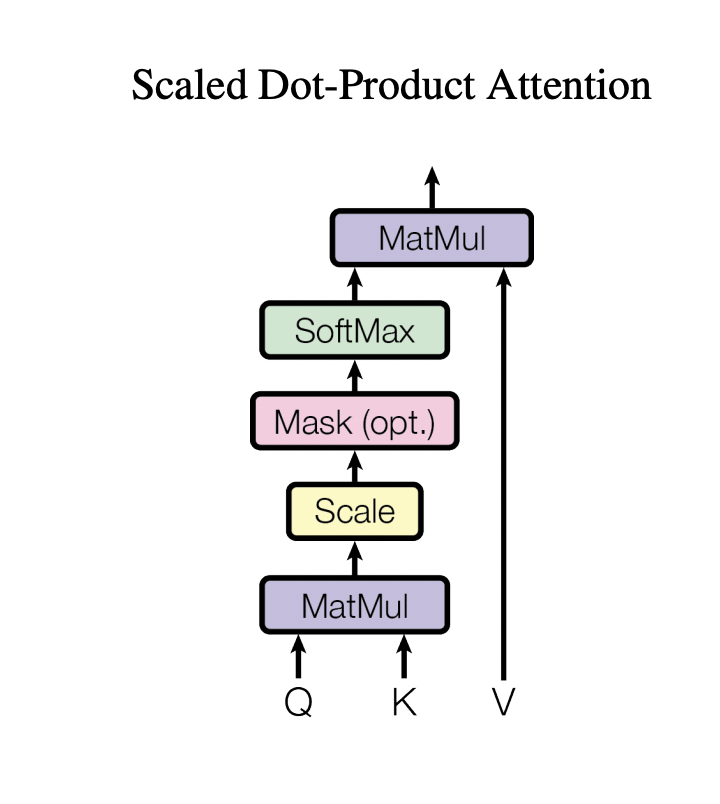
In a standard transformer encoder, we use a mechanism called self-attention. We have an input embedding that goes through three different linear transformations (generally which are learnable) in order to create the query, key, and value vectors. We the do a matrix multiplication $QK^T$, and then scale it by $\frac{1}{\sqrt{d_k}}$. We then compute the softmax($\frac{QK^T}{\sqrt{d_k}}$) and then do one final matrix multiplication with the value vector softmax($\frac{QK^T}{\sqrt{d_k}})V$.

def self_attention(query, key, value):
    dim = key.shape[-1]
    # (Query * tranpose(key)) / sqrt(dim)
    scores = torch.bmm(query, key.transpose(-2, -1)) / sqrt(dim)
    weights = F.softmax(scores, dim = -1)
    return torch.bmm(weights, value)

The output tensor of a self-attention has the shape of [bs, L, L] where bs is the batch size, and L is the number of tokens in the sequence length. As you can see self-attention is $O(n^{2})$ in both time and space complexity, because each token needs to attend to every other token in the sequence. Because of this, large language models that use traditional self-attention require an enormous amount of compute and memory in order to compute long sequences.

Linformer

The Linformer paper (Wang et al. 2020) introduced a methodology for self-attention with linear complexity.

In this paper, they claim that self-attention is approximately low rank. (While the paper includes a couple proofs that would be too complicated to work through for an introduction, it’s definitely worth checking out. Heres a good video that works through the proofs)

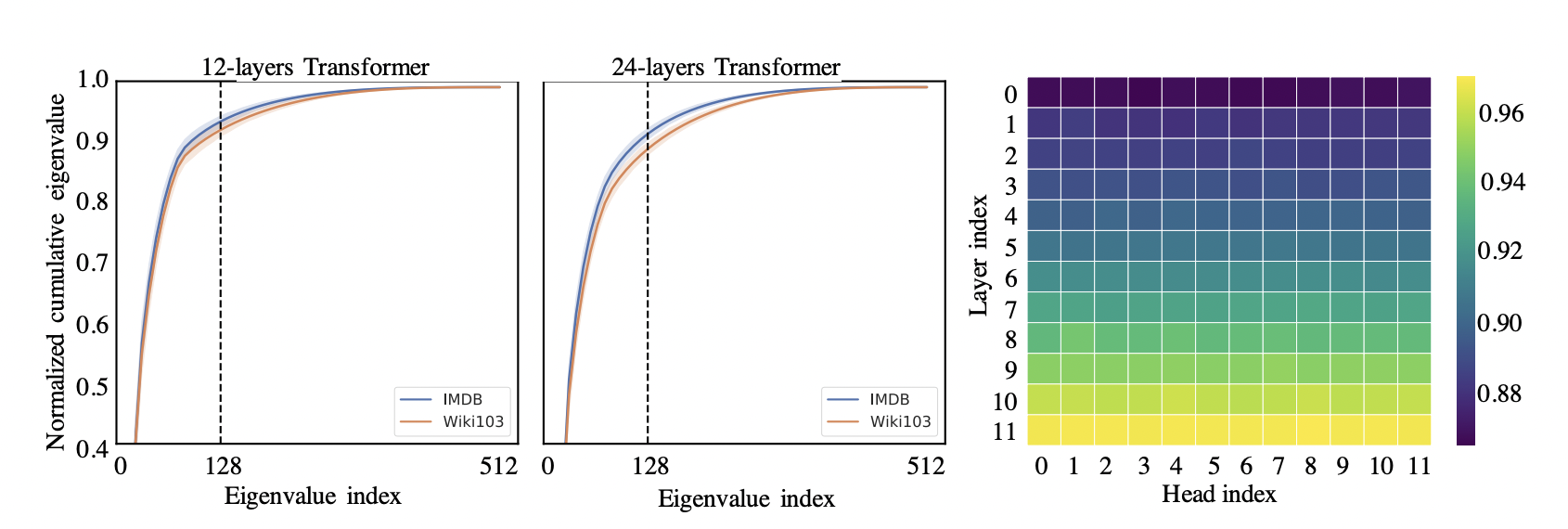
Here the author’s do an empirical look into the RoBERTa models, and applied a singular value decomposition (SVD), where they found that normalized cumulative singular value had long-tail distribution, essentially meaning that the majority of the information was stored in only a few layers. They found that distribution of the singular values in the higher layers was more skewed, meaning that the information is concentrated in only the largest singluar values, and the rank of the matrix softmax($\frac{QK^T}{\sqrt{d_k}})$ is low rank.

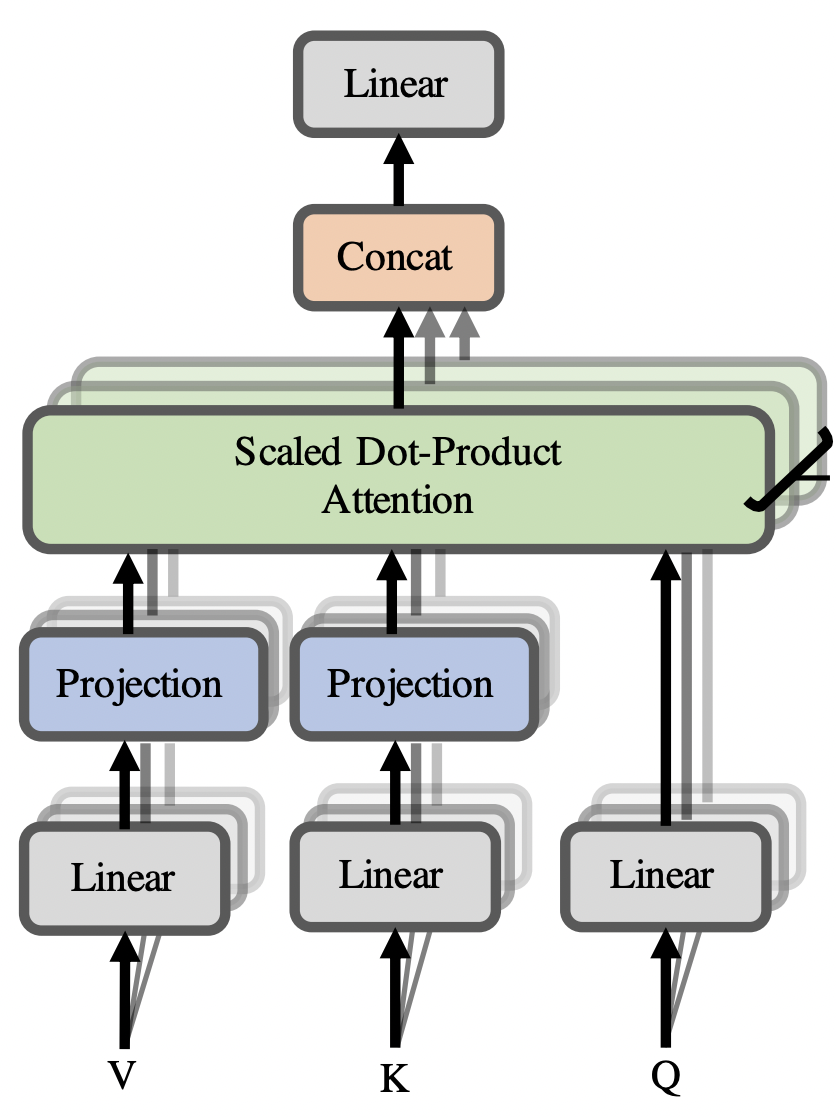
Linear attention is computed as softmax($\frac{Q(E_iK^T)}{\sqrt{d_k}})F_iV$, where $E_i,F_i \in \mathbb{R}^{n x k}$ are linear projections which we use to down-project our key and value vectors (to a lower dimension) when computing self-attention. This allows us to compute an $(n x k)$ matrix instead of an $(n x n)$ matrix which gives $O(nk)$ runtime. It’s worth noting that $E_i$ and $F_i$ are generally fixed projection matrices, and not learnable.

They suggest to choose $k$ such that $k = min(\Theta(9dlog(d)/\epsilon^2),5\Theta(log(n)\epsilon^2))$ with $\epsilon$ error. Since $k$ doesn’t depend on the sequence length, and is treated as a constant, the runtime of linear self-attention is therefore $O(n)$.

The authors also experiment with different types of parameter sharing between the projection matrices. They used headwise sharing, where $E_i$ and $F_i$ are shared between every head within the same layer. They used key-value sharing where they use headwise sharing, but the projection matrices where they use $F_i = E_i$, so each key and value vector gets down projected by the same matrix $E_i$. Lastly they tried layer-wise sharing where they used the same projected matrix $E_i$ for every $E_i$ and $F_i$ projection across every head and every layer.

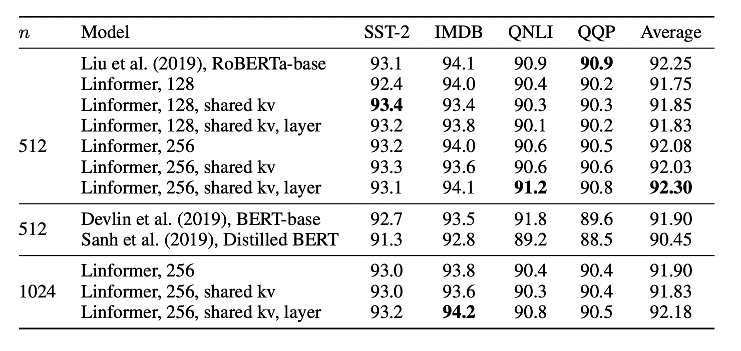
The results end scoring only about half a point below than RoBERTa, which seem to show a lot of promise for the actual performance of the model.

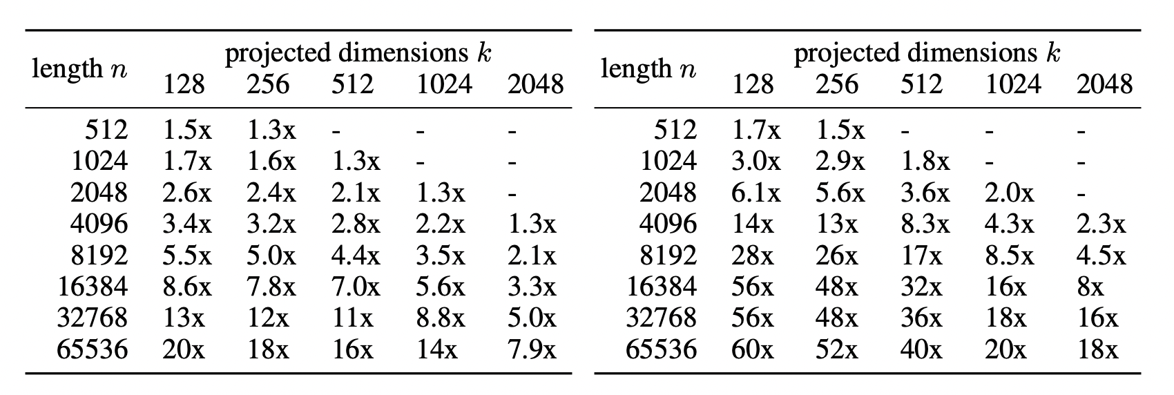
The real difference comes when the authors compared the linformer(diagram shows linformer with layer-wise sharing) vs a standard transformer(not specified in the paper). The left table is time saved during inference, and the right table shows memory saved. As we can see, we get a massive speed up, even at small sequence lengths, despite only a marginal decrease in performance vs RoBERTa.

Reformer

The Reformer (Kitaev et al. 2020) identified three areas of transformer inefficiency:

1) Memory in a model with $N$ layers has to store $N$-times more activations than that of a single layer network.
2) The depth $d_{ff}$ (hidden dimension) of the feed forward networks is generally much larger than than the depth $d_{model}$ (embedding dimension), which results in very high memory use.
3) Standard self-attention is computed in $O(n^2)$ time and space complexity where $n$ is the sequence length, because each token needs to attend to every other token.

1) We can solve the problem of having $N$ blocks activations by using Revnets (Gomez et al. 2017). Standard residual connections require us to store activations during the forward pass which we then use to compute the gradients during the backward pass. Reversible residual connections allow us to reconstruct the activations of the current layer from the activations of the previous layer. Reversible networks works by having inputs $(x_1,x_2)$ such that $(x_1,x_2) \mapsto{(y_1,y_2)}$, where $(y_1, y_2)$ is the output.

$y_1 = x_1 + F(x_2)$ $y_2 = x_2 + G(y_1)$.

Using these formulas, we can compute the activations needed for any layer during backpropagation by simply subtracting the residuals instead of adding them like in a traditional resnet.

$x_2 = y_2 - G(y_1)$ and $x_1 = y_1 - F(x_2)$

The Reformer incorporates Revnets with the attention and the feed forward network and move the layer norm inside the residual blocks.

$Y_1 = X_1 + Attention(X_2)$ and $Y_2 = X_2 + FeedForward(Y_1)$

Reversible residual connections allow us to only storea activations for one layer, instead of $N$ layers.

2) The authors of the paper deal with large memory usage from the feed forward network by chunking the computation into $c$ chunks.

$Y_2 = [Y_2^{(1)};…;Y_2^{(c)}] = [X_2^{(1)} + FeedForward(Y_1^{(1)};..; X_2^{(c)} + FeedForward(Y_1^{(c)})] $

Since we can compute feed-forward layers independent across positions (unlike self-attention) we perform computation on one chunk at a time. Note that this does slow down the network, since we usually batch the operations together to make use of GPUs, but processing one chunk at a time helps reduce the memory required.

3) The third problem deals with approximating self-attention. We can accomplish through locality-sensitive hashing (LSH). Why locality-sensitive hashing for approximating self-attention? As we know the reason self-attention is $O(n^2)$ is because of $softmax(QK^T)$ creates a matrix of size [batch_size x seq_len x seq_len]. But we also know that taking the softmax of $(QK^T)$ makes it so that the largest elements dominate the matrix and almost every element will be squished to almost 0. LSH allows us to consider a small subset of say 32 or 64 keys, that are most similar to our key, and attend to only this subset of 32 or 64 keys.

Okay, but how does LSH work? LSH is an efficient way to do a nearest neighbor search in a high dimensional vector space. We take a hash function $h(x)$ and an input vector $x$, and we pass $x$ through our hash function, and $x$ gets placed in a bucket. The goal of LSH is to place vectors that are similar in the same bucket, and vectors that aren’t similar in different buckets.

In standard self-attention, we use three separate linear projections to project our input vector $x$ into the query, key, and value vector. In LSH, we share the linear projection between the $K$ and $Q$, so our $K$ vector $ = Q$ vector. We define our hash function as $h(x) = max([xR;-xR])$, where $R$ is a fixed random projection matrix of size $[d_k,b/2]$ where $xR$ and $-xR$ are concatenated together. Once we’ve hashed our vectors, vectors only need to attend to other vectors that are in the same bucket, as opposed to in standard self-attention where every vector has to attend to every other vector.

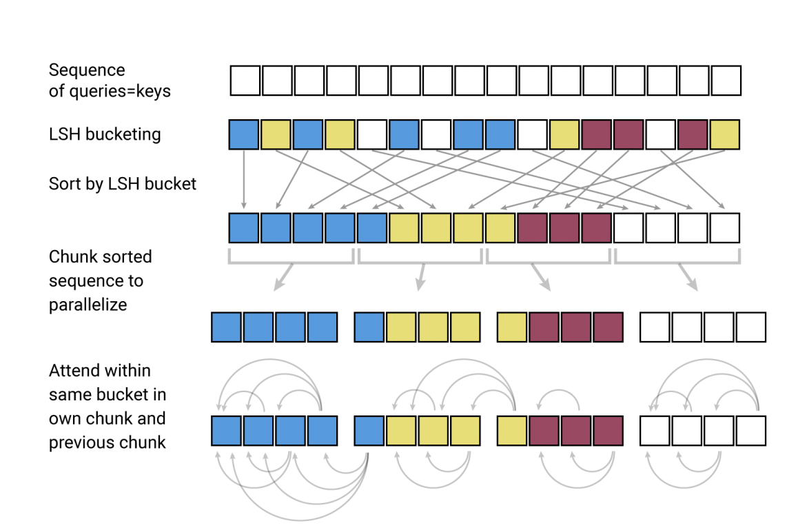
LSH attention can be formalized given a query position $i$ as

$o_i = \sum_{j \in{P_i}} $$exp(q_i * k_j - z(i, P_i))v_j$ where $P_i = \{j: i\geq{j}\}$

$P_i$ represents the set that the query at position $i$ attends to, and $z$ denotes the partition function(the normalizing term in the softmax). This form of self-attention is still scaled by $\sqrt{d_k}$, it’s just omitted by the authors for clarity.

They then employ the use of multi-round hashing, where we hash for $n_{rounds}$ to reduce the likelihood that similar vectors get placed in separate buckets. This improves the performance of the model at the expense of more computation required.

It’s also worth noting that during causal language modeling, the authors of the paper masked not only the future words, but, also masked words from attending to itself, unless only there was no other word to attend to, like the first token in a sequence.

Retroformer

RETRO (Retrieval-Enhanced TransfOrmer)(Borgeaud et al. 2021) is a retrieval based transformer that uses a separate database to perform lookups. The advantage of having an outside query-able database means that we don’t need to store all the information within our model’s parameters and can rely on a database “lookup” to augment extra information. For example, if we were to deploy a transformer based model for QA to cover the news, we wouldn’t need to re-train often in order to update the network’s “knowledge”, instead we could just update the database. This also means that we don’t need an absurdly large model such as GPT-3’s 175 billion parameters, and can rely on a much smaller model which we could fine-tune on 1 GPU. The smallest version of Retro is ~150 million parameters, which is slightly larger than BERT-base. Retro is also promising because we can use pre-trained models, and augment them with a database (hence the name).

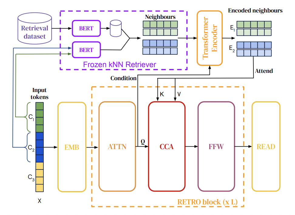
Okay, but how does this work under the hood? RETRO is made up of both an encoder stack and a decoder stack (like the original transformer paper). They also create a key-value database made up of frozen BERT embeddings (i.e they take the information they want to store (which are chunks of tokens) and pass it into the database as a BERT embedding). Using frozen BERT embeddings means that they don’t need to recompute embeddings later on. The key-value pairs are stored as
[$N$, $F$], where $N$ is the neighbor chunk used to compute the key and $F$ is the continuation in the original document. We can compute $BERT(N)$ by simply passing chunk $N$ through BERT, and taking the chunk embedding output and averaging it. Here $BERT(N)$ represents the averaged embedding of a chunk found in the database. We can the compute $BERT(C)$ where $C$ is a chunk computed from our input and not from the database and compute an approximate $k$-nearest neighbor search by taking the $L_2$ distance of the two vectors.

$d(C,N) = \Vert BERT(C) - BERT(N) \Vert_2^2$

The model retrieves the two nearest neighbors and their continuations ($F$). Using the ScaNN library, they’re able to query 2 trillion tokens in only 10 ms.

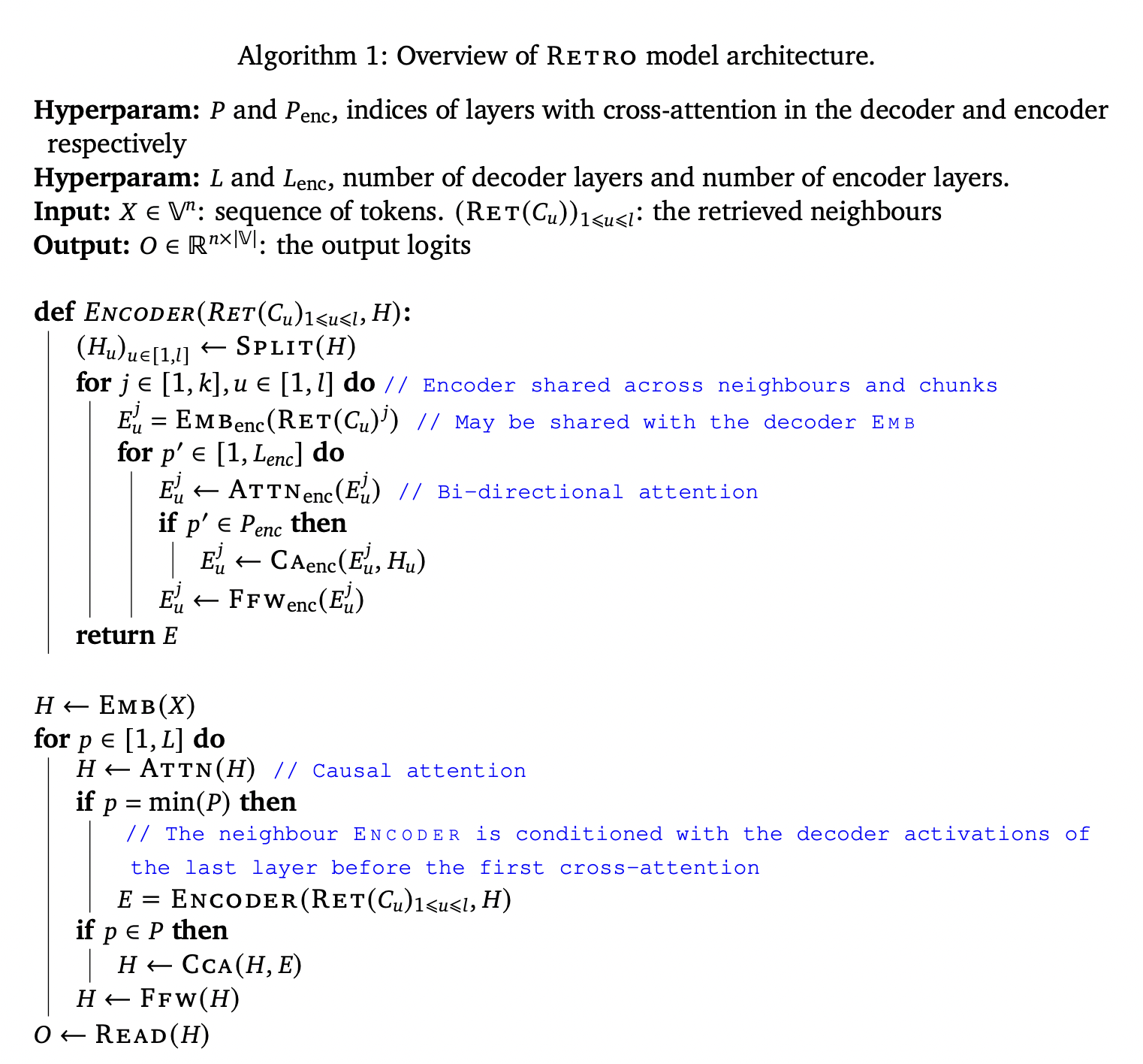
While this seems like a lot, we can see that the RETRO encoder is actually quite similar to the diagram. We take two inputs $H$, which is an intermediate activation and $RET(C_u)_{1\leq u \leq l}$, which are the retrieved neighbors. We take $H$ and chunk it, and then first compute the embeddings. We only chunk and compute the embeddings once, right at the beginning, regardless of the number of encoders. We then go through each layer of the encoder, first computing the bi-directional attention of each embedding $E_u^j$, then compute the cross-attention of the $E_u^j$ and $H_u$ which is an intermediary of the last token in chunk $C_u$. We then take the computed value and pass it through a final feed forward network return the output of that.

Cross-attention differs from self-attention because in self-attention, the query, key, and value vectors all come from the same input vector after applying a linear projection.

The decoder stack is made up of a standard transformer decoder (like one found in GPT), and interweaves a RETRO decoder between every 3rd layer starting at layer 9. Here we take an input embedding $X$ and apply causal mask (i.e can’t look at future words/tokens) to get output $H$. When we reach the first RETRO block, we take the activation $E$ from the final layer of the encoder. FOr every subsequent RETRO block that we hit, we compute the chunked cross-attention of $H$ and $E$. At the end of each block (for both the standard decoder and RETRO decoder), we process the output with a feed forward network. Once we’ve iterated through all the layers of the decoder, we can get our output logits which we can push through a softmax to get our probability distribution of our next word choice.

RETRO opens up a whole new field, where the authors experimented with RETROfitting pre-trained models, and saw a boost in performance. Check out the original paper where they addressed much more in depth about training and evaluating the performance of the model, especially with regard to test set leakage. RETRO is able to achieve GPT-3 level performance with 25x fewer parameters.

It’s also worth checking out OpenAI’s (WebGPT), which is a GPT based transformer model with a database.