CSE 142 - Machine Learning Notes
Key ML concepts
An ML system is a task requires an appropriate mapping - a model - from data described by features to outputs. Obtaining such a model from training data is called a learning problem.
Bayes Rule: $P(X|Y) = \frac{P(Y|X)(P(X)}{P(Y)}$
- Usually framed in terms of hypotheses $H$ and data $D$
- $P(H_i|D) = \frac{P(D|H_i)(P(H_i)}{P(D)}$
- Posterior probability (causal knowledge) = $P(H_i|D)$
- Likelihood (diagnostic knowledge) = $P(D|H_i)(P(H_i)$
- Prior probability = $P(H_i)$
- Normalizing Constant = $P(D)$
Geometric model: use intuitions from geometry such as separating (hyper-)planes, linear transformations, and distance metrics
Probabilistic models: view learning as a process of reducing uncertainty, modelled by means of probability distributions
Logical models: are defined in terms of easily interpretable logical expressions
Grouping models: divide the instance space (the space of possible inputs) into segments, in eah segment a different (perhaps very simple) model is learned
Grading models: learning a single, global model over the instace space
There are predictive and descriptive ML tasks.
- Predictive tasks aim to predict/estimate a target variable from some features.
- Descriptive tasks are concerned with exploiting underlying structure in the data and finding patterns.
Features
ML models are trained on features, which are measurements performed on instances.
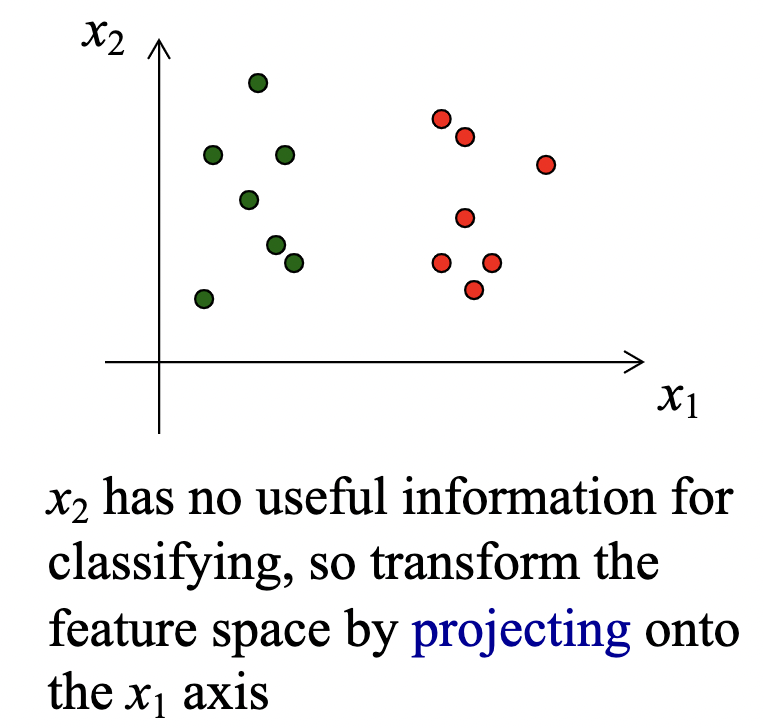
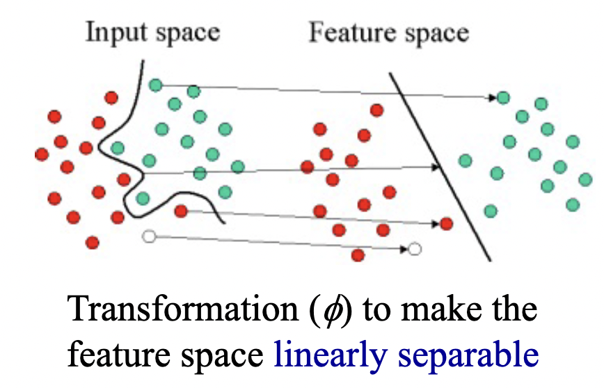
A common first step in ML problems is to transform the features into a new feature space. We want features that encapsulate the key similarities and differences in the data, are robust to irrelevant parameters and transformations, and have a high signal-to-noise ratio.
We perform dimensionality reduction on features that are useless or redundant (have correlations with other features).
The intrinsic dimensionality of (N-dimensional) data describes the real structure of the data, embedded in N-space.
Logical Models
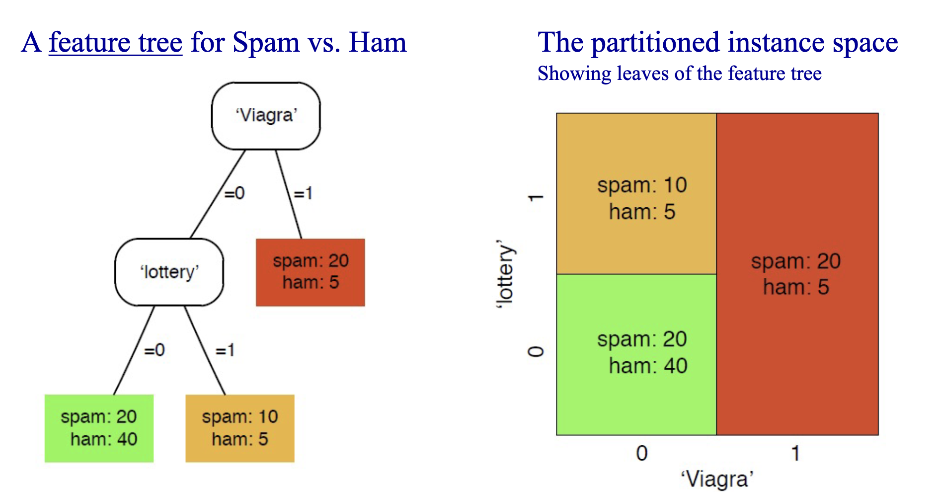
Logical models focus on the level of human reasoning and are much more easily human-understandable. They’re often represented as feature trees that iteratively partition the instance space (space of all posible inputs). We call feature trees whose leaves are labelled with classes as decision trees.
Classification
Regression
Regression learns a function (the regressor) that is a mapping from $\hat{f} : X \to \mathbb{R}$. We generally estime a regression function based on the residual, $r(x) = f(x) - \hat{f}(x)$.
Scoring and Ranking
A scoring classifier is a mapping $\hat{s}: X \to \mathbb{R}^k$ along with a class decision based on these scores. Scoring classifiers assign a margin $z(x)$ to each instance $x$ such that $z(x) = c(x)\hat{s}(x)$. $z(x)$ is positive when \hat{s} is correct and negative if \hat{s} is incorrect. Large positive margins are good and large negative margins are bad.
We can use the scores from the scoring classifier as rankings. We note that the magnitude of the scores is “meaningless”, but the order of the scores isn’t.
Class probability estimation
A class probability estimator is a scoring classifier that outputs probabilites over the $k$ classes. $\hat{p}: X \to [0,1]^k$, where $\sum_{i = 1}^{k}\hat{p}_i(x) = 1$. In ML, we classify relative frequencies
Linear Models
Linear models are geometric models for which regression or classification tasks create linear (lines, planes, hyperplanes(N-dimensional planes)) decision boundaries.
- $ y = f(ax_1 + bx_2) = af(x_1) + bf(x_2)$
- in matrix form $\to$ $y = Mx + c$
Linear models are useful for functions that are approximately linear, are simple and easy to train, math is tractable, and avoid overfitting issues. Linear models are prone to underfitting, especially when the underlying data isn’t linearly or approximately linear.
Linear least-regression
The residual($\epsilon$) is the difference between the label($f$) and our output($\hat{f}$).
- $\epsilon = f(x_i) - \hat{f}(x_i)$
Linear least-regression minimizes the sum of the squared residuals. $\min \sum_{i=1}^{D} \epsilon_i^2$. To minimize our loss function, we take partial derivatives to optimize the parameters of our model.
Ex: Find the relationship between height($h$) and weight($w$).
- linear model $\to$ $w = a + bh$
- set the partial derivatives (w/ respect to $a$ and $b$) to 0 and solve for $a$ and $b$.
- $\frac{\partial}{\partial a}\sum_{i = 1}^{n}(w_i - (a + bh_i))^2 = -2\sum_{i = 1}^{n}(w_i - (a + bh_i)) = 0 \to \hat{a} = \bar{w} - \hat{b}\bar{h} $
- $\frac{\partial}{\partial b}\sum_{i = 1}^{n}(w_i - (a + bh_i))^2 = -2\sum_{i = 1}^{n}(w_i - (a + bh_i))h_i = 0 \to \hat{b}\large\frac{\sum_{i = 1}^{n}(h_i - \hat{h})(w_i - \hat{w})}{\sum_{i = 2}^{n}(h_i - \hat{h})^2} $
- regression model becomes
- $ w = \hat{a} + \hat{b}h = \bar{w} + \hat{b}(h - \bar{h})$
Multivariate linear regression
For multiple $N$ input variables, we represent linear regression in matrix form $y(x) = w^Tx +w_o$.
As an example if we have $y_i = w_2x_{i2} + w_1x_{i1} + w_0x_{i0} + \epsilon_i$
We’d have the function $y = Xw + \epsilon$.
Optimizing this function takes the form of $w^* = \underset{w}{argmin}(y - Xw)^T(y-Xw)$
- $y$ represents the predicted labels $y = \begin{bmatrix} y_1 \\ y_2 \\ \vdots \end{bmatrix}$
- $X$ represents the data in homogenous form
\(X =
\begin{bmatrix} x_{12} & x_{11} & x_{10} \\\
x_{12} & x_{11} & x_{10} \\\
\vdots & \vdots & \vdots\
\end{bmatrix}\)
- $w$ represents the regression parameters
\(w =
\begin{bmatrix}
w_2 \\\
w_1 \\\
w_0
\end{bmatrix}\)
- $\epsilon$ represents the residuals
\(\epsilon =
\begin{bmatrix}
\epsilon_1 \\\
\epsilon_2 \\\
\vdots
\end{bmatrix}\)
We use regularization in order to avoid overfitting by adding a regularization function.
- $w^* = \underset{w}{argmin}(y - Xw)^T(y-Xw) + \gamma r(w)$
- $\gamma$ is a scalar amount demterining the amount of regularization.
Nonlinear kernel classifiers
In problems where a linear decision boundary isn’t sufficient, we can adapt our linear methods to some nonlinear decision boundaries by transforming the data nonlinearly to a feature space in whcih linear classification can be applied. The kernel trick is a way of mapping features into another (often higher dimensional) space to make the data linearly separable, without having to compute the mapping explicitly.
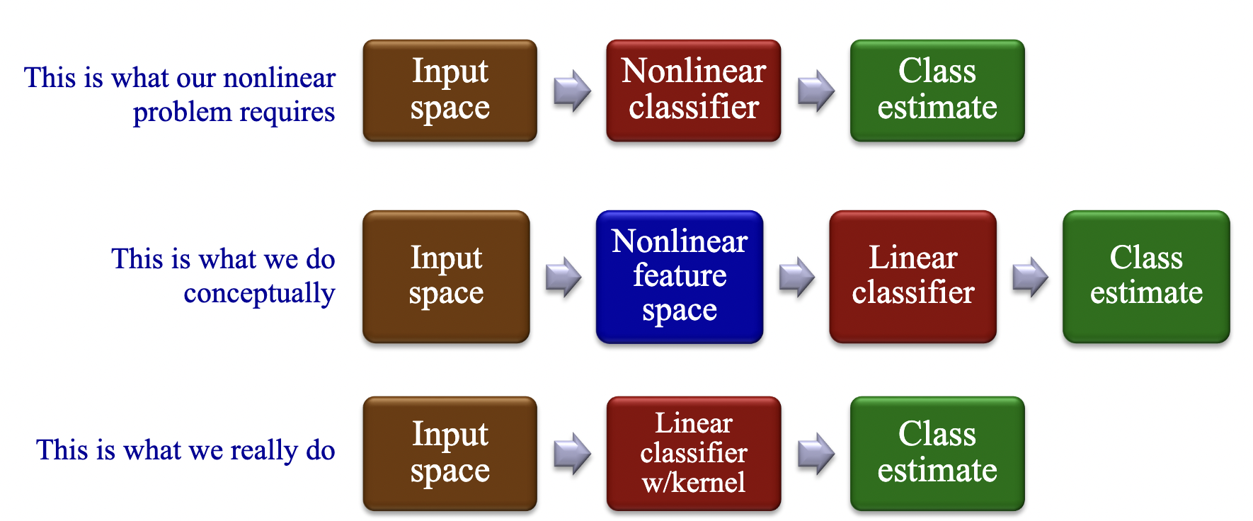
We do this by replacing the dot product operation in a linear classifier $x_1 * x_2$ with a kernel function $k(x_1, x_2).
There is no absolute way to find the mapping that will make the data linearly separable, it requires insight into the data and trial and error.
Common kernel functions include:
- the linear kernel: $k(x_1, x_2) = x_1^T x_2$
- the polynomial kernel: $k(x_1, x_2) = (x_1^Tx_2 + c)^d$
- the gaussian kernel: $k(x_1, x_2) = exp(\frac{-\parallel x_1 - x_2 \parallel^2}{2\sigma ^ 2})$
Distance and clustering
We often use distance as a measure of similarity. The most common distance metrics are:
- $L1$ distance (Manhattan): $d(x,y) = \sum_{i=1}^d \mid x_i - y_i \mid$
- $L2$ distance (Euclidian): $d(x,y) =\; \mid\mid x - y \mid\mid \;= (\sum_{i=1}^d (x_i - y_i)^2)^{1/2}$
- $L_p$ distance (Minkowski): $d(x,y) = (\sum_{i=1}^d (x_i - y_i)^p)^{1/p}$
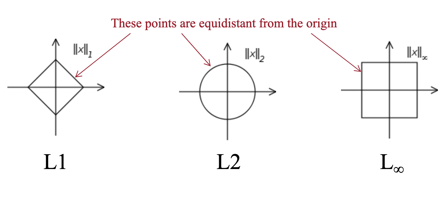
We measure the distances of a data point to either an exemplar or neighbor.
- exemplar: a prototypical instance (generally the mean) instance of a class
- neighbor: a “nearby” istance or exemplar
K-Nearest Neighbor classifiers
We classify the new instance $x$ as the same class as the nearest labeled exemplar ($k = 1$). We use k-NN classification when we take a majority vote for the $k$ nearest neighbors. We can use a vote among all neighbors within a fixed radius $r$ or we can combine the two, stopping when (count > k) or (dist > r).
Determining which dinstance method to use depends on the problem at hand. Odd values of k are generally preferred to avoid ties.
Clustering
The goal of clustering is to find clusters (groupings) that are compact with respect to the distance metric. We use distance measures as a proximity for similarity. As a result, we want to find clusterings such that intra-class similarity is high (small distance between points) and low inter-class similarities (large distance between clusters).
To build our Scatter matrix, we need to build $X_z$, a zero-mean covariance matrix.
- For column vectors where $X_z$ is a matrix that holds all the zero-centered samples: $\frac{1}{k}X_zX_z^T = \frac{1}{k}S$
- For row vectors where $X_z$ is a matrix that holds all the zero-centered samples: $S = X_z^TX_z$
Features
Quantitative features: These features are measured on a meaningful numerical scale and its domain is often real values. Ex: weight, height, age, etc
Ordinal features: These features we only care about the ordering, not the scale and its domain is an ordered set. Ex: rank, street addresses, preference, ratings, etc
Categorical features: These features have no scale or order information and its domain is an unorder set. Ex: colors, names, part of speech, etc

Feature Engineering
We can construct new features that can be constructed from our current given feature set.
Principal Component Analysis
Principal Component Analysis constructs new features that are linear combinations of given features. We do this by computing the eigenvectors and eigenvalues and use the to perform dimensionality reduction to find the intrinsic linear structure in the data.
$PC_1 = \underset{y}{argmax}(y^TX)(X^Ty)$
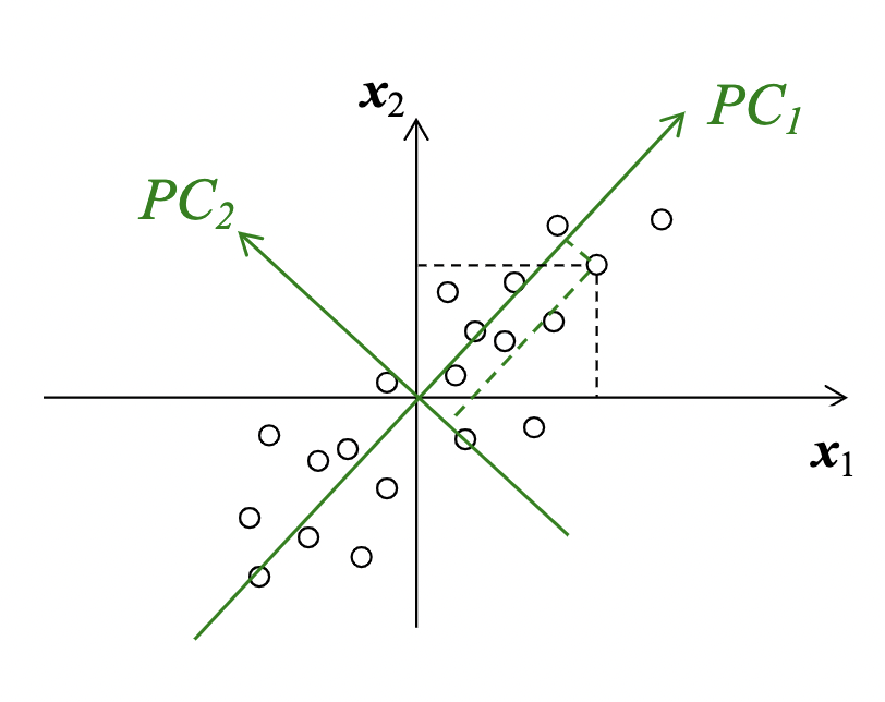
The first principal component is the direction of maximum (1D) variance in the data.
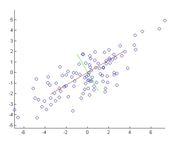
The second principal component is the direction of maximum variance orthogonal to the first PC. This holds true for all additional PCs, and for N-dimensional data, there can be N principal components. But only a subset $k$ PCs are useful, we are able to perform dimensionality reduction.
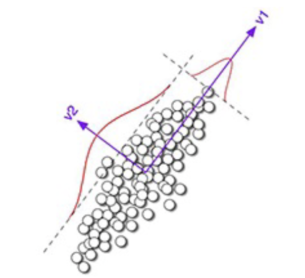
Note: we compute the PCA on zero-mean data (subtract the mean from each data point to have zero-based centroid).
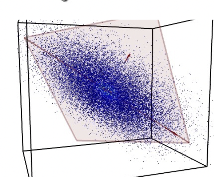
Ex: For $n$ points of a dimension $d$ let $X = \begin{bmatrix}x_1 &x_2 & … & x_n \end{bmatrix}$($d$x$n$)
- We can use the scatter matrix $S = X_ZX_z^T$ ($d$ x $d$) to measure variance
- The eigenvectors of S are the principal components of the data, ordered by decreasing eigenvalues
$Su_i = \lambda_i u_i \to SU = U\Lambda \equiv S = U\Lambda U^T $(eigendecomposition), where $U$ is the matrix of eigenvectors (columns of U) and $\Lambda$ is a diagonal matrix of eigenvalues diag($\lambda_i, \lambda_2, …, \lambda_d$).- the eigenvector $u_i$ associated with the largest eigenvalue $\lambda_i$ is the first principal component.
- if rank(S) < d, then some eigenvalues will be 0.
Eigenvalues can give clues to the intrinsic dimensionality of the data, and gives us a way to efficiently approximate high-dimensional data with lower-dimensional feature vectors.
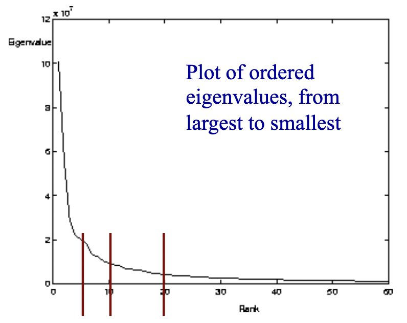
Above is 60-dimensional data (60 eigenvectors and eigenvalues). The small eigenvalues mean that their associated eigenvectors don’t contribute much to the representation of the data, so we can choose some arbitrary cutoff, like the first 5, 10, or 20 eigenvectors.
Ensembles
We can combine multiple models to increase performance at the cost of increased complexity. Generally this is done by constructing multiple different models from adapted versions of the training data (ex rewighted or resampled) and combine the predictions of the models(ex averaging, voting, weighted voting, etc).
Bagging
Bootstrap aggregation is way creating $T$ different models trained on different random samples of the training data set. Each sample is a set of training data, called a bootstrap sample. Generally we boostrap sample by randomly sampling the dataset with replacement (meaning the same data point can be chosen multiple times) so that the size of our bootstrap sample is equal to the size of our dataset.
Random forest ensemble is a popular bagging method, which is an ensemble of decision tress, where each tree is built on both a subset of the total features and on bootstrapped samples.
Bagging is a variance reduction technique (inrease consistency).
Boosting
Boosting is similar to bagging, but differentiates by iteratively generating the new training set by giving extra weight to the misclassifications of the previous classifiers.
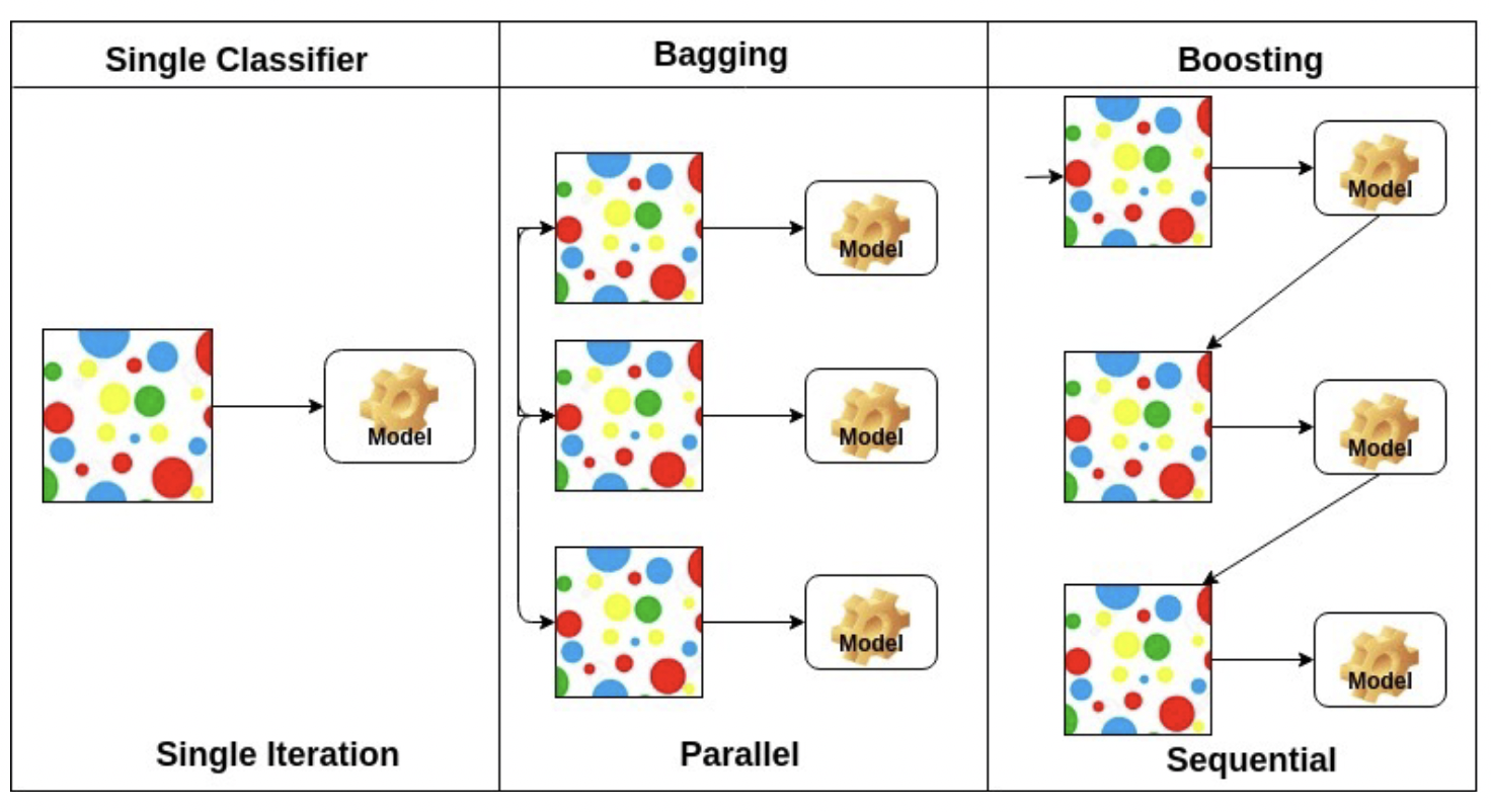
The intuition behind boosting is simple: we start off with a weak classifier, and for data points we get wrong, we increase their weight, and for data points we get right, we decrease their weights, so our next weak classifier will perform better on our misclassifications.
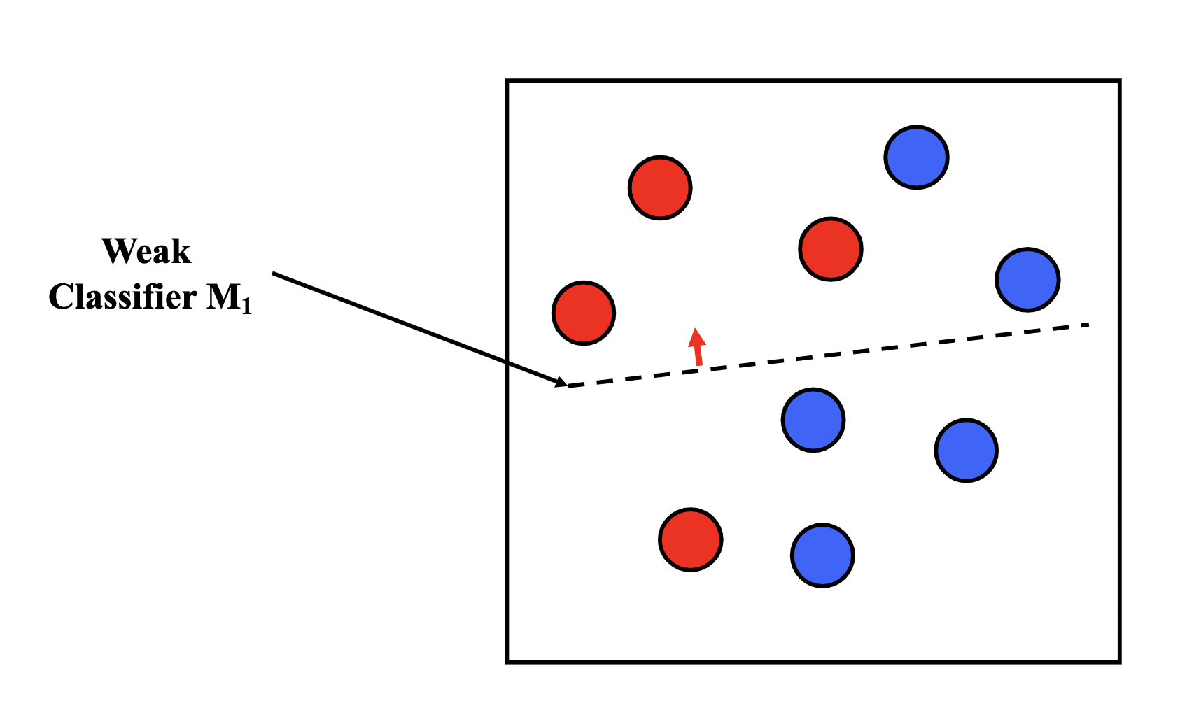
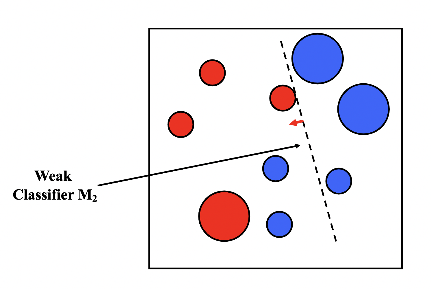
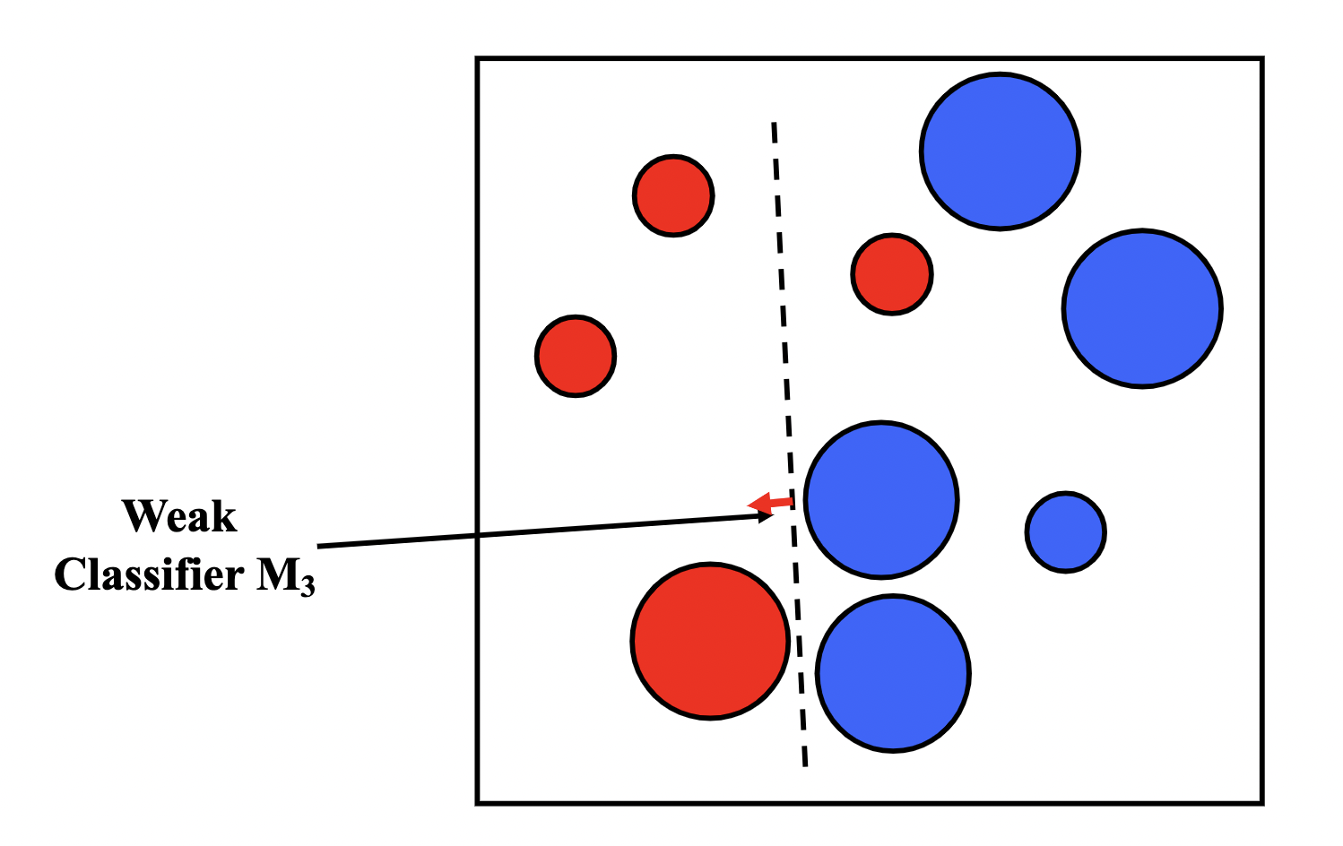
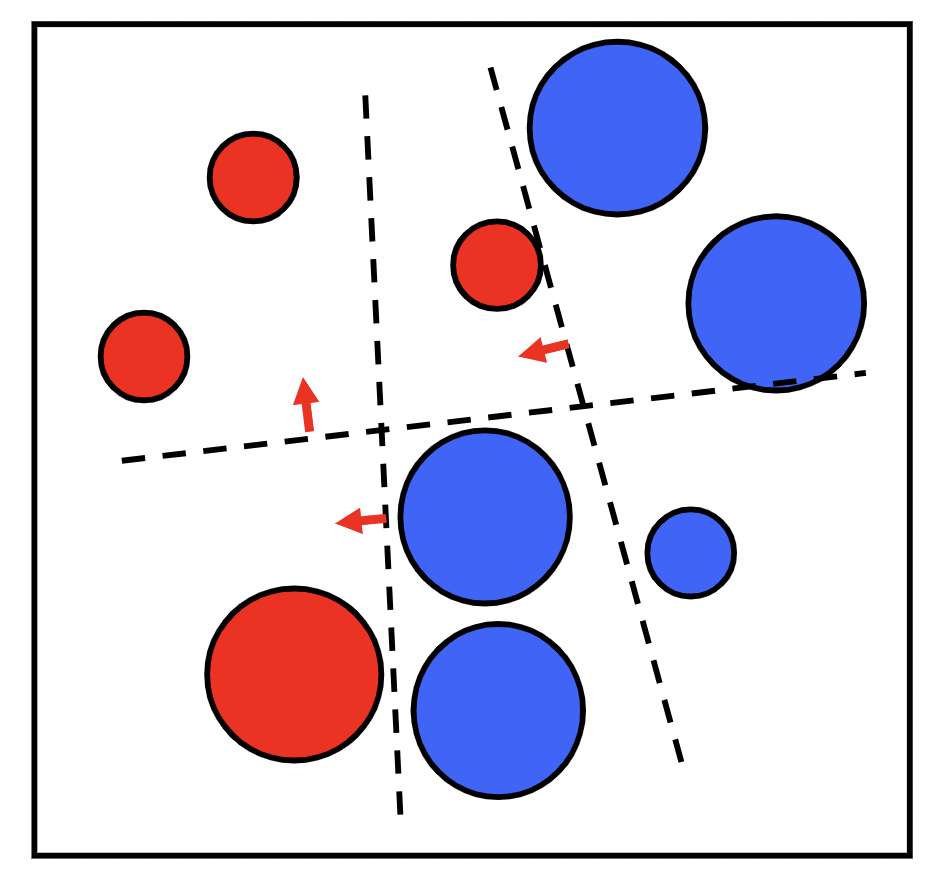
We then assign an $\alpha_t$ for each $T$ model in our ensemble as a representation of how confident we are in that model. The prediction of our ensemble is a weighted vote $\sum_{t=1}^{T}\alpha_tM_t(x)$.
We assign the confidence factor $\alpha_t$ based on the error $\epsilon_t$ ${\large\alpha_t = \frac{1}{2}ln\frac{1 - \epsilon_t}{\epsilon_t}} $
Boosting is a bias reduction technique (increase accuracy).