Designing Machine Learning Systems Notes

General ML System Design

ML systems need to be reliable, scalable, maintainable and most importantly solve a business metric (such as click-rate).

When developing reliable models, we want our systems to perform correctly to some desired level of performance. Unlike traditional software, ML models tend to fail silently, where detecting failures in production are much harder to catch than 404s or runtime errors. If a google translate translation is incorrect, how can Google find this issue?

Our systems need to be scalable. Our usage rate might peak at 1 million queries per hour, but bottom out at 100,000 queries during off-hours. We need to be able to scale our systems as traffic fluctuates. We also will need to be able to scale up the number of models we have in production, where each model serves a different use-case/customer. We need to be able to deal with all the different models with artifact management to monitor their performance.

Our systems need to be maintainable and adaptable. Models need to be reproduceable and failures in the system need to be easily diagnosable. ML systems need to be adaptable, since they’re part code and part data, and data can change very quickly.

Iterative Process

• Step 1: We need to scope out our project, and see what our business needs are and what are stakeholders want from a business perspective.
• Step 2: We need to take our raw data, and transform it, by handling the different formats, cleaning it, and sampling and generating our labels.
• Step 3: We need to extract the features from our model, and develop our ML algorithm. This stage involves the most ML knowledge and requires model selection, training, and evaluation.
• Step 4: We deploy our model to our users.
• Step 5: We need to monitor our model for performance decay and other related metrics, and to continously “adapt” our model.
• Step 6: Re-evaluate our model performance w.r.t. our business goals and analyze our business insights. In a general workflow, we might have a system for process raw data into features, and another service that takes those features and inputs them into an ML model.

Data Engineering

Data models define how the data stored in a particular data format is structured. Data models describe the data in the real world and databases specify how the data should be stored on machines. We generally have two different methods of data passing: historical data in data storage engines, and streaming data in real-time transports.

Data Sources

One source of data is user input data, such as text, images, videos, uploaded files, etc. This type of data is the most prone to malformed input data, (think uploading wrong files, google translate with random text, etc). This data requires the most processing and checking. Another example of user-generated example is logging their behavior, such as their clicks, how long they spend looking at something, etc.

System generated data is data generated by the system that includes various logs and system outputs. These are mainly used for debugging.

There are also internal databases, which manage their assets such as inventory, customer relationship, users, and more.

The final one is third party data, where a company might track a user’s Apple unique id, IDFA. This kind of data is getting more and more locked down, with more government regulation.

Data Format

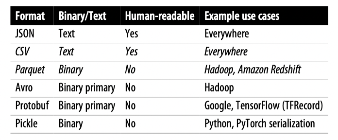
The two most common types of data storage are CSV, which are row-major column format (consecutive elements in a row are stored next to each other in memory), and parquet, which is column major, which means means consecutive elements in a column are stored next to each other.

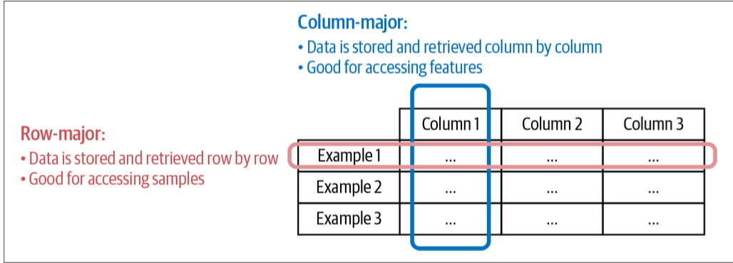
We want to use row-major when we do alot of writes (ie adding new examples as new rows). We want to use column-major format when we need to do alot of column based reads (ie accessing a subset of features quickly).

Using binary vs text is more efficient in both size and for compressing/decompressing necessary files.

Relational Model

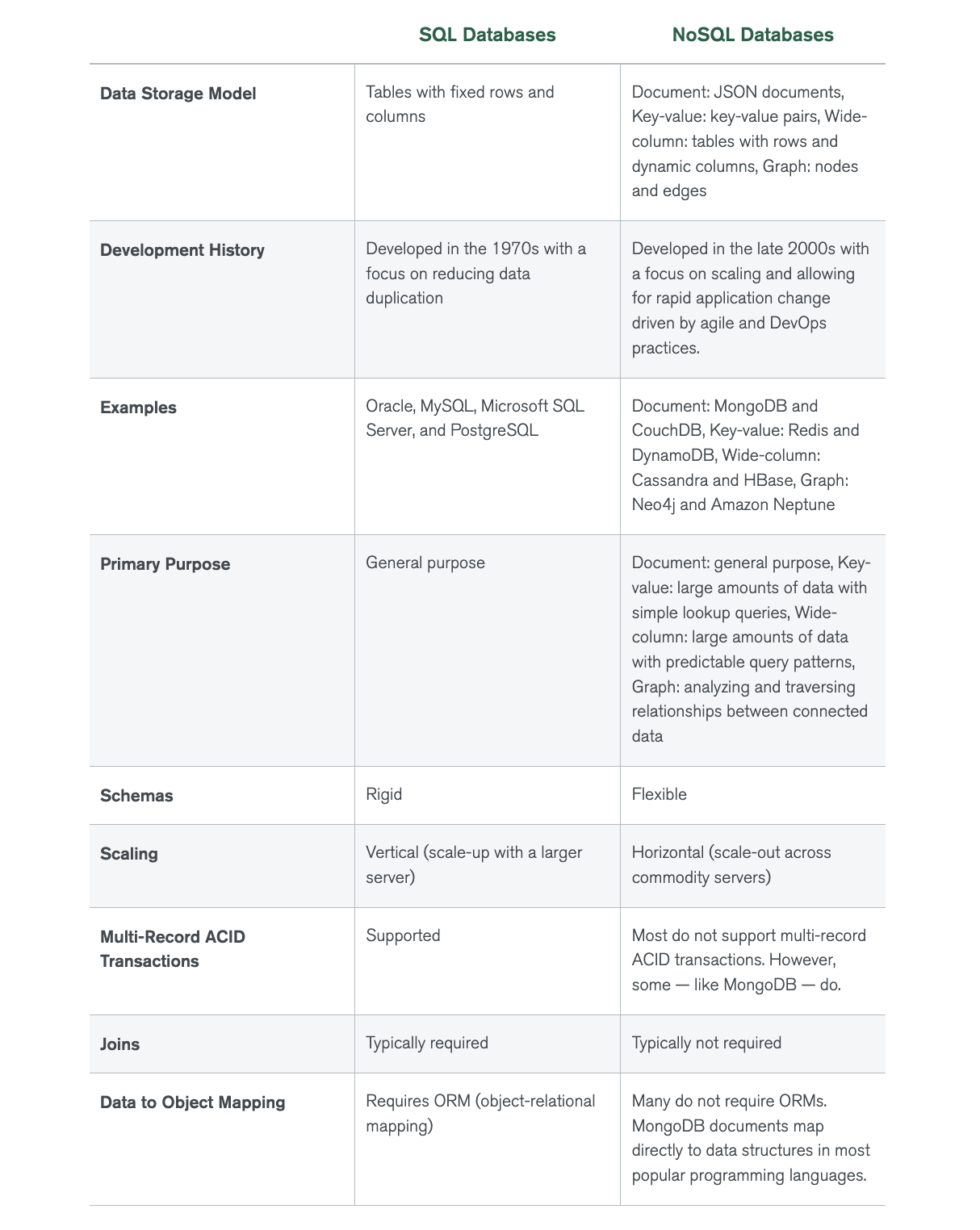
Data is organized into relations; each relation is a set of tuples. A table is an accepted visual representation of a relation, and each row of a table makes up a tuple. Relational models use SQL for queries. It’s important to note that SQL is a declarative language, where you specify the outputs you want, and the computer figures out the steps needed to get you the queried outputs. These models require following a very strict schema and schema management is painful.

NoSQL

The benefit of NoSQL is that it doesn’t restrict us to a certain schema (and schema management is very painful!).

There are two main kinds of NoSQL models: document model and graph model. The document model is built around the concept of “document.” A document is often a single continuous string, encoded as JSON, XML, or a binary format like BSON (Binary JSON). All documents in a document database are assumed to be encoded in the same format. Each document has a unique key that represents that document, which can be used to retrieve it. It does this by shifting the responsibility of assuming structures from the application that writes the data to the application that reads the data.

The graph model is built around the concept of a “graph.” A graph consists of nodes and edges, where the edges represent the relationships between the nodes. A database that uses graph structures to store its data is called a graph database. If in document databases, the content of each document is the priority, then in graph databases, the relationships between data items are the priority.

Structured vs Unstructured Data

There are two kinds of data, structured and unstructured. Structured data follows a pre-defined schema, making data very easily to analyze. The disadvantage of structured data is that updating a schema requires updating the data within the schema as well.

Unstructured data doesn’t follow a predefined schema, but it still might contain intrinsic patterns that help with extracting features. This allows us to store data with any type or format and we can just convert our data to bytestring.

A data warehouse is a repository for storing structured data. A data lake is a repo for storing unstructured data.

Data Storage and Processing

Data formats and data models specify the interface for how users can store and retrieve data. Storage engines, also known as databases, are the implementation of how data is stored and retrieved on machines.

Transactional and Analytical Processing

Online transaction processing (OLTP) is the process in which transactions (tweets, uber orders, etc) are inserted as they are generated, and are occasionally updated when something changes, or deleted when they are no longer needed. These actions are stored in transactional databases, which generally fulfill the low latency, high availability requirement (since they’re generally customer facing).

• Transactional databases generally fulfill ACID (atomicity, consistency, isolation, durability).
  • Atomicity: A property in databases where all steps in a transaction are completed. If any step fails, than all other steps should fail. If someone requests an uber, and payment is declined, than don’t order a car.
  • Consistency: To guarantee that all transactions should follow predefined rules. Ie a transaction should only be able to be made by valid users.
  • Isolation: To guarantee that all transactions happen at the same time as if they were isolated. Ie two users shouldn’t be able to book the same driver.
  • Durability: To guarantee that even after a transaction has been committed, it’ll remain committed even in the case of a system failure. A ride should still come even if your phone dies.

ETL: Extract, Transform, Load

When data is extracted from different sources, it’s first transformed into the desired format before being loaded into the target destination such as a database or a data warehouse. The extract phase is where we extract the data we want from our data sources and reject the data that we don’t want (malformed, corrupted, etc). During the transform phase, we do the vast majority of our processing. We apply our data transformations including but not limited to transposing, deduplicating, sorting, aggregating, deriving new features, more data validating, etc. The load phase describes how and how often we want to load our data into our target destination.

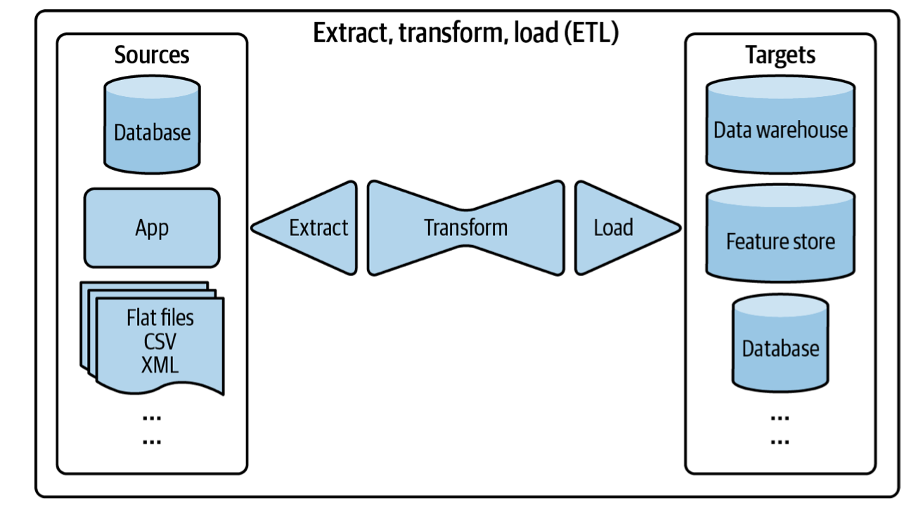
ETL is attractive because it allows for the fast arrival of data since there’s little processing needed before data is stored. As the amount of data we have scales the less efficient (and less attractive) this solution becomes since it requires searching through a massive amount of raw data.

Modes of Dataflow

Data Passing through Databases

Process A writes to a database and process B reads from said database. While the simplest, you need to make sure that both processes have access to the database and read/write operations are generally slow, so latency is an issue.

Data Passing through Services

Process A sends a request to process B that specifies the data that process A wants, and process B returns the requested data over the same network. This is called request-driven. The most popular styles of requests used for passing data through networks are REST (representational state transfer) and RPC (remote procedure call). One major difference is that REST was designed for requests over networks, whereas RPC “tries to make a request to a remote network service look the same as calling a function or method in your programming language.” Because of this, “REST seems to be the predominant style for public APIs. The main focus of RPC frameworks is on requests between services owned by the same organization, typically within the same data center. Request-driven data passing is synchronous: the target service has to listen to the request for the request to go through.

Data Passing Through Real-Time Transport

A piece of data broadcast to a real-time transport is called an event. This architecture is, therefore, also called event-driven. In this kind of event, we use a middle-man called a broker for our other services to send and receive data.

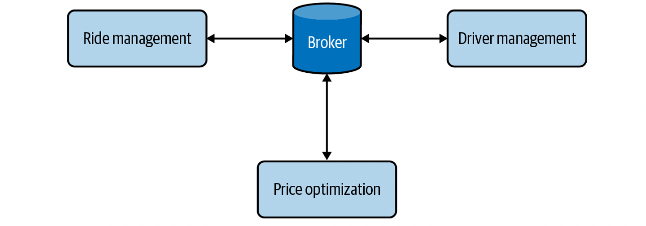
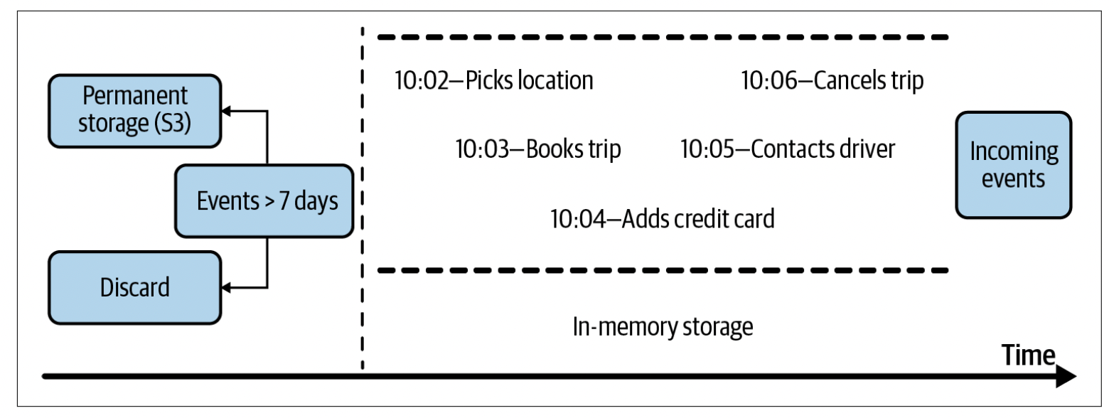
Pubsub is a type of a real-time transport which is short for publish-subscribe. In the pubsub model, any service can publish to different topics in a real-time transport, and any service that subscribes to a topic can read all the events in that topic. The services that produce data don’t care about what services consume their data. Pubsub solutions often have a retention policy— data will be retained in the real-time transport for a certain period of time (e.g., seven days) before being deleted or moved to a permanent storage (like Amazon S3).

In a message queue model, an event often has intended consumers (an event with intended consumers is called a message), and the message queue is responsible for getting the message to the right consumers.

Batch Processing vs Stream Processing

Batch processing is when we process data in batches, where we use systems like MapReduce and Spark for efficiency. This technique is more useful when dealing with data who’s features change less frequently. Stream processing is processing data when it comes in. This technique is more useful when we need to compute features that change frequently.

Data and feature quality assessment

We care about data, not datasets. Datasets denote a set that is finite and stationary, while data in production is neither.

Sampling

• Non-probability sampling is when the selection of data isn’t based on any probability criteria
  • convenience: sample of data based on availability
  • snowball: future sampling is based on existing sample: ie scrape twitter users and sample all the people they follow
  • judgment sampling: experts decide what to sample
  • Quota sampling: sample based on quotas for certain groups
• Probabilistic sampling:
  • simple random sampling: give all samples from a population equal chance of being selected. Under-represented samples may not be accurate
  • stratified sampling: separate population into stratas (individual groups you care about), and perform simple random sampling from each strata $\to$ each group will be represented
  • weighted sampling: each sample is given a weight, which determines the probability of it getting sampled
• Importance Sampling: Allows us to sample from a distribution when we only have access to another distribution.
  • We sample $x$ from distribution $P(x)$, but for some given reason $P(x)$ is difficult or impractical to sample from. We can sample $x$ from distribution $Q(x)$, and weigh the sample $\frac{P(x)}{Q(x)}Q(x)$.
• Reservoir Sampling: Imagine you have an incoming stream of tweets, but you want to sample a certain $k$ number of them. You don’t know the probability of a certain tweet being sampled, so you want to make sure that every tweet has an equal probability of being selected, so that at any give time when you stop the algorithm, the tweets are of the correct probability.
  1. Put the first $k$ elements into a reservoir
  2. For each incoming $n$th element, generate a random number $i$ such that $1 \leq i \leq n$
  3. If $1 \leq i \leq k$: replace the $i$th element in the reservoir with the $n$th element. Else, do nothing.

Labels

Natural labels are tasks where labels are determined on some given action. For example, recommendation systems when someone clicks on a particular item or not.

Hand labeling: Very expensive, especially where subject matter expertise is required (X-ray scans for example). Hand labeling also poses a threat to data privacy when dealing with sensitive information that shouldn’t leave an organization. Third, hand labeling is extremely slow, imagine transcribing every word for a speech.

Label Multiplicity: When labeling data and using multiple sources as annotators, how do you deal with the issue of label mismatch/disagreement? First, identify a clear problem definition to reduce the likelihood that annotators disagree on rules. Secondly, you can also use data lineage, which tracks the origin of each data sample and its corresponding label, which can help flag potential biases in our data.

Weak supervision: Leverage (often noisy) heuristics to generate labels. Generally a small number of ground truths/labels are recommended to guide the development of heuristics. Examples of heuristics, built around the idea of labeling functions include the following:
- Keyword heuristics, where if something contains a keyword, it’s filed into a certain label.
- Regular expressions, such that if a note matches (or doesn’t match) a certain regex.
- Database lookup, where if our query returns a successful/unsuccessful hit.
- Output of other models

This method is useful when you only need a small, cleared subset of data to write your labeling functions, so this can be especially useful when data has strict privacy requirements. The benefit of this is that you can re-use your labeling functions for new data (adaptive) or across different teams. We use machine learning models instead of just relying on the output of our heuristics because the ML models can generalize much better than our labeling functions.

Semi-supervision: leverages strucutural assumptions to generate new labels based on a small set of initial labels. A common approach to this is to use self-training, where you use your prediction as a label on the training data for data that was previously unlabeled. Another popular method is to do perturbation on your data (small changes that shouldn’t affect the real label) to augment your data.

Active learning: is the process of labeling samples that are the most useful according to some heurestic. An example is labeling predictions that fall under some threshold in the uncertainty.

Class Imbalance

Class imbalance usually results in insufficient signal for a model to detect minority classes since it essentially relies on few-shot learning to determine whether something belongs to a minority class or not. Another reason is models are much more likely to get stuck in a non-optimal solution by learning a simple heuristic instead of learning something useful about the underlying structure of the data. The final reason is asymmetric costs of error, where if you don’t adjust your loss function accordingly, than inaccurately predicting $x$ as $y$ is significantly more costly than misclassifying $y$ as $x$.

Dealing with class imbalance involves

• choosing the right metrics for your problem
• data-level methods (changing the data distribution to make it less imbalanced)
• algorithm-level methods (make it more robust to class imbalance)

Metrics

Using the right evaluation metrics is the first step to dealing with class imbalance. If you’re developing a model to detect cancer, and there is a 1:99 ratio of positive to negatives, than a model that always predicts negative will have a 99% accuracy despite being useless.

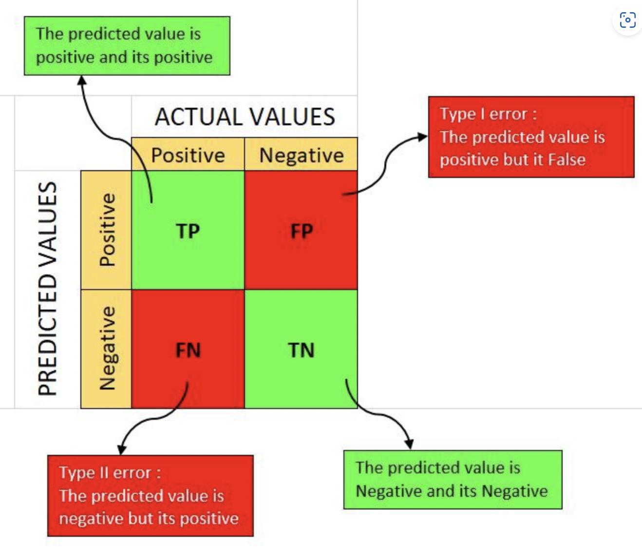
We can compute the recall or the true positivity rate as $\frac{TP}{P}$ and we can compute the precision as $\frac{TP}{\hat{P}}$. We can compute the F1 score as $\frac{2 * precision * recall}{precision + recall}$ or as $\frac{2 * TP}{P + \hat{P}}$.

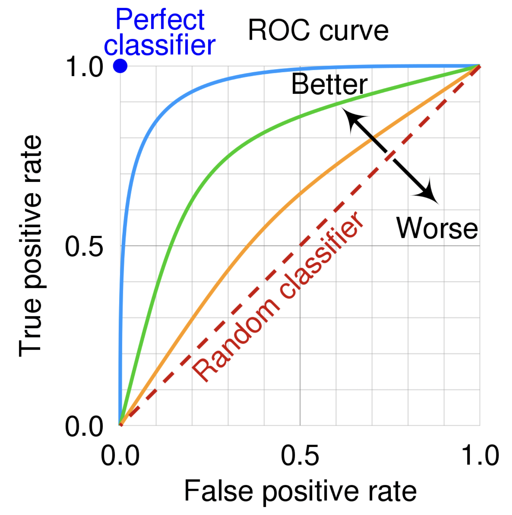
If we have a model (on binary classification), we can treat it as a regression problem, where we predict the positive class above a threshold of $.5$ and negative below or equal to $.5$. We can adjust the threshold to increase the recall (TPR) while reducing the FPR.

We can use an ROC curve (Receiver Operating Characteristic) to see how well our model performs on only the positive class.

Data level methods

You have two methods for resampling your data, either undersampling your majority class, or to oversample from your minority class. Undersampling runs the risk of losing important data, since you’re removing information, and oversampling runs the risk of overfitting your model to the data. You can make use of two-phase learning, where you train the model on the resampled data, fine-tune on the original dataset. Another method is dynamic sampling, where you oversample the lower performing class and undersample the high performing class during training.

Algorithm level methods

Algorithm level methods are designed to make the algorithm more robust to class imbalance. These generally tend to changing the loss function. The loss of a function can be defined as $L(X;\theta) = \sum_{x}{L(x;\theta)}$, where every prediction on the loss function is treated as equal.

THe first thing you can use is cost-sensitive learning, where misclassification of different classes incur different cost. It’s modeled as $L(x;\theta) = \sum_{j}{C_{ij}P(j \mid x;\theta)}$, where you manually define the cost matrix of $C_{ij}$. We can make use of class-balanced loss, where we assign a smaller weight to over-represented classes and assign a larger weight to under-represented classes. We can define a simple function as $W_i = \frac{N}{number \ of \ sample \ of \ class \ i}$. We can define the loss as $L(x;\theta)= W_i\sum_{j}{P(j \mid x;\theta) Loss(x;j)}$. One loss function that we can use that works really well with class imbalance is focal loss.

Data Augmentation

Data augmentation is a simple of way of increasing the amount of training data which makes models more robust to noise and adversarial attacks.

The simplest form of data augmentation are simple labeling-preserving augmentation methods, like cropping, flipping, rotating, etc a picture of something (in the case of computer vision classification). An NLP equivalent is substituting words out with words that are similar meaning semantically (generally by using some distance metric). An extension of this is perturbation, which relies on “tricking” NNs by creating noisy images for performing adversarial attacks to improve robustness.

Feature Engineering

Having the right features will generally lead to better performance than techniques like hyper-parameter tuning. The promise of deep learning is that it promises to no longer engineer features, but this isn’t always the case. An example of feature engineering before deep learning on NLP involved text processing such as expanding contractions, removing punctuation, and lowercasing everything. The disadvantage of this is that it requires domain knowledge, and is error prone. Feature engineering is the process of choosing what to use and extracting the information you want.

• An example of this is on a twitter thread (for detecting spam), you might take into effect:
  • the comment: who posted it, how many likes/retweets it has
  • the user: when the account was created, how active it is, how many likes/retweets it has, the number of followers/following
  • the thread: how many impressions it has (more popular posts see more spam)

Techniques of Feature Engineering

Handling Missing Values

Missing data is one of the most common things that occures in ML at the production level. Let’s assume we have the following table where we’re given the task to predict if someone will buy a house in the next year.

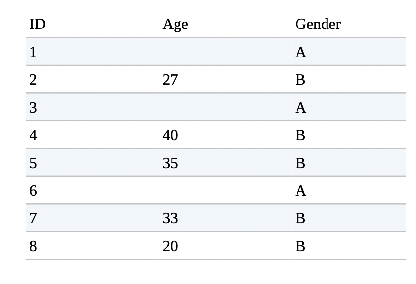
There are 3 types of missing data:

1. Missing not at random (MNAR): The reason a value is missing is because of the value itself. Some people may omit the gender, income to avoid being potentially discriminated against.
2. Missing at random (MAR): When the reason a value is missing is due to another observed variable. For example, age values may be omitted frequently with gender “A”.
3. Missing completely at random (MCAR): The most rare kind of missing variable, where the data is missing at random, with no pattern.

The easiest remedy (but not always the best) is deletion. The first kind is column deletion, where if a variable has too many missing values, you can just remove it. The downside is that you might be removing key information (for example, if you remove marital status from house buyers, but married couples are significantly more likely to buy a house). The alternative is row deletion, where if an example has a missing value(s), then just remove the example. This works well when the missing values are MCAR, and when the total percentage of data removed is small. The downside of this is if the missing values are MNAR, and as a result, you’re deleting key information.

The alternative to deletion is imputation, the process of filling in missing values with certain values. One simple solution is to plug in the default value(0 for ints, “” for strings, etc), the downside of this is that it can cause bugs, if for example a model never saw 0 for a certain feature. Another approach is filling the missing data with the mean, median or mode value. If it’s a categorical feature, than you can choose a random or the most common category. The downside of imputation is adding noise and/or data leakage.

Scaling

Going back to the house analogy, if we have two ages (20 and 40), and two incomes (10,000 and 150,000), the model won’t be able to understand the difference between 150,000 and 40, and might give priority to the larger number for outcome prediction. Feature scaling is a way of scaling your values to be between $(0,1]$ (the range $[-1,-1]$ also tends to work out quite well). Other feature scaling things you can do is normalizing your data (to a standard distribution -zero mean and unit variance).

Discretization

Discretization is the process of turning a continous feature into a discrete feature. We can do this by creating buckets for the given values. A common example is age demographics where you might have an age group under 18, 18-25, 25-35, etc. The benefit of this is that instead of infinite number of inputs, our model only needs to deal with a much lower, finite number of categories.

Encoding Categorical Features

Let’s assume we’re creating a recommendation system on Amazon for shoppers. A naive thing to assume is that the categories that we’re working with are static, because they aren’t. Let’s say we have 1 million companies in a category, and we train our model, but when we push it to production, we realize that new companies that the model hasn’t seen in training performs extremely poorly. So we decide to add a new variable UNKNOWN, where we list all unknown companies into. The issue is that since our model hasn’t seen UNKNOWN, it has no idea how to recommend any product from UNKNOWN.

The solution to this is the hashing trick, where you use a hash function to generate a hashed value for each category. We use the hashed values as the index of that particular category. The only issue becomes with hash collisions, but in practice, the performance loss is minimal.

Feature Crossing

Feature crossing is the technique to combine two or more features to generate new features. This technique is most useful to model non-linear relationships between features. Feature crossing is essential for models that can’t learn non-linear relationships, such as linear regression and decision trees. An example for predicting house buying would be feature crossing isMarried and numChildren (isMarried, numChildren).

Data Leakage

Data Leakage refers to the phenomenon when a form of the “label” leaks into the set of features used for making a prediction, and this same information is not available during training. An example of data leakage -

---

Suppose you want to build an ML model to predict whether a CT scan of a lung shows signs of cancer. You obtained the data from hospital A, removed the doctors’ diagnosis from the data, and trained your model. It did really well on the test data from hospital A, but poorly on the data from hospital B. After extensive investigation, you learned that at hospital A, when doctors think that a patient has lung cancer, they send that patient to a more advanced scan machine, which outputs slightly different CT scan images. Your model learned to rely on the information on the scan machine used to make predictions on whether a scan image shows signs of lung cancer. Hospital B sends the patients to different CT scan machines at random, so your model has no information to rely on. We say that labels are leaked into the features during training.

---

• The following are the most common reasons for data leakage:
  • Splitting time-correlated data randomly instead of by time. The canonical example of this is analyzing stock prices, where you want to train on the first 6 days, and evaluate the model on the 7th day of data. If you randomly split, than some data from the 7th data will “leak” into the training set.
  • Scaling before splitting. Scaling your data requires global information about your dataset, and if you scale before splitting, than your leaking information from the test dataset (like the mean) into the training set, which allows the model to adapt by leaking information it shouldn’t be seeing.
  • Filling in missing data with statistics from the test split. Similar to the point above, make sure to split and then fill in missing data with only the specific set’s standard mean, median, etc.
  • Poor handling of data duplication before splitting: Check for duplicates before splitting, or else you’re contaminating your validation/test set.
  • Group leakage: A group of examples have strongly correlated, but are divided into different splits. A patient has two CT scans, taken a week apart, but both end up in different sides of the split.
  • Leakage from collection processes: Going back to the example of where the CT scans are different based on the machine, this kind of leak requires a deep understanding of how the data is collected and potential subject matter expertise.

Detecting Data Leakage

Measuring how each feature or a set of features are correlated to a target variable, and investigating whether the correlation makes sense or not. If adding a new feature significantly improves performance, than either that feature was very good or there’s data leakage.

Model Development

Choosing the loss function is based on the model type and whether labels are available or not. An example for unsupervised learning, K-means clustering uses the variance within the data points in the same cluster as its loss function.

Choosing ML models

We first need to frame our ML problem. Is the task a classification or a regression problem? Most regression problems can be framed as classification problems (house prediction price bucketed into price groups) and classifications as regression problems (if a value is >.5 it belongs to the positive class else negative). Are we dealing with binary or multiclass classification. Are we dealing with multilabel classification (an example can belong to multiple classes).

Decoupling Objectives

• Let’s assume our goal is to build a recommendation system to rank user’s feed. We have three goals in mind:
  • Filter out spam
  • Filter out NSFW content
  • Rank posts on engagement: how likely a user is to click on it

After building our model we quickly realize that optimizing for user’s engagement alone leads to questionable and potentially unethical recommendations, so we redefine our goal as to maximize user engagement while minimizing the spread of misinformation and extreme views. So in addition to our previous goals, we add the following two:

1. Filter out misinformation.
2. Rank posts by quality.

We now have two metrics that we one to optimize for: quality_loss, which is the difference between the predicted quality of a post and its actual quality, and engagement_loss, which defines the difference between each post’s predicted clicks and its actual clicks. One such function we can use to model our loss is as follows loss = $\alpha$ quality_loss $+ \beta $ engagement_loss. We can then test out values for $\alpha$ and $\beta$ until we reach a satisfactory performance metric. The downside is that for everytime we tune $\alpha$ and $\beta$, it might increase one and decrease the other, meaning that we need to retrain our model.

Another approach that we can use is to train two separate models, one model that optimizes to minimize engagement_loss and another to minimize quality_loss. We can then combine the outputs of the two models $\alpha$ quality_loss $+ \beta $ engagement_loss, where we can adjust $\alpha$ and $\beta$ independently, without retraining our models.

A general rule of guidance is if there are multiple objectives, we should decouple them as it makes model development and maintenance easier. Besides not having to retrain your model to do small tweaks, we might need to update one model more frequently than another (say we have one to determine if something is spam [update frequently] and one to determine quality [update less frequently]).

Evaluating ML Algorithms

When we select a model(s) for our problem, we don’t focus on every type of model, but only a subset that are suitable for our problems. An example is classify tweets, we can try traditional ML methods such as Naive Bayes or linear regression, or more DL methods such as using BERT or other transformer variants. If we want to build a system to detect fraudulent transactions, we can re-frame the problem as a classic abnormality detection, we can use k-nearest neighbors, isolation forest, clustering, and neural networks.

When choosing a model we have to keep in mind that different algorithms require different amount of labels and compute power. There are tradeoffs to be made for inference vs training speed. Interpratibility is also something me we might want to have based on our business needs.

• Here are some tips to decide what ML algorithm to employ.
  • Avoid SOTA: SOTA models are generally only evaluated on academic datasets, so its performance isn’t guaranteed to be better on our datasets. These models are probably more expensive, more complex, or take longer to implement than other non-SOTA models.
  • Start with simplest model: Simpler models are easier to deploy, and deploying your model early allows you to validate that your prediction pipeline is consistent with your training pile. Secondly, starting with something simple and adding more complex components step by step makes it easier to understand your model and debug it. Lastly, it serves as a baseline to compare to more complex models. A common misconception is that simplest means least effort. An example of this is using off the shelf NLP solutions from huggingface to get easy, well-performing SOTA models for relatively low effort.
  • Avoid human biases in selecting model. Make sure that you test each model equally (in terms of experimenting), and don’t just blindly favor the “cooler” model.
  • Evaluate good performance now vs good performance later: Take into account potential improvements of a model in the future, and the ease/difficulty of achieving the improvements.
  • Trade-offs: Understand what’s more important in the performance of an ML system. An example is do we want to prioritize false positives or false negatives. Another common trade-off is latency vs accuracy, google search would be better with higher latency due to a better/more complex model powering it, but would dissuade users from searching so frequently.
  • Understanding your model’s assumptions: Understanding what assumptions a model makes and whether our data satisfies those assumptions can help you evaluate which model works best for your use case.
    • Prediction assumption: every model that predicts an output $Y$ from input $X$ make the assumption that its possible to predict $Y$ from $X$.
    • IID: NNs assume that examples are picked independently and identically distributed from the same distribution.
    • Smoothness: Every supervised machine learning method assumes that there’s a set of functions that can transform inputs into outputs such that similar inputs are transformed into similar outputs. If an input $X$ produces an output $Y$, than an output close to $X$ would produce an output proportionally close to $Y$.
    • Tractability: Let $X$ be the input $Z$ be the latent representation of $X$. Every generative model makes the assumption that it’s tractable to compute the probability $P(Z\mid X)$.
    • Boundaries: A linear classifier assumes that decision boundaries are linear.
    • Conditional independence: A Naive Bayes classifier assumes that the attribute values are independent of each other given the class.
    • Normally distributed: many statistical methods assume that data is normally distributed.

Ensembles

Ensembling is a popular method for improving performance. Each model is considered a base learner, and the outputs are aggregated together and used to predict an outcome. Ensemble methods are more complex and harder to maintain, so they’re more advisable to use where small performance gains matter alot (click rate in ads).

Ensembles perform better when the base learners are as uncorrelated as possible (because high correlation means the models will make very similar predictions). The goal of ensembling is built upon the premise that each model will make mistakes, but the mistakes will be different from each model, so aggregating the results will give better results.

There are three major ways of ensembling: bagging to reduce variance, boosting to reduce bias, and stacking to boost generalization.

Bagging: (shortened from bootstrap aggregation) - Given a dataset, instead of training one classifier on the entire dataset, you sample with replacement to create different datasets, called bootstraps, and train a classification or regression model on each of these bootstraps. Sampling with replacement ensures that each bootstrap is independent from its peers. If we’re doing classification, we do majority vote, and for regression we take the average.

Bagging has the most positive effect on unstable methods, such as NNs, trees, and subset selection in linear regression. It degrades performance on stable methods such as K-NNs. An example of bagging is random forest.

Boosting:Boosting is a family of iterative ensemble algorithms that convert weak learners to strong ones. Each learner in this ensemble is trained on the same set of samples but the samples are weighted differently among iterations. As a result, future weak learners focus more on the examples that previous weak learners misclassified.

• The general process for boosting goes as follows:
  • start with a weak learner trained on the entire dataset
  • Samples are reweighted based on how well the first classifier classifies them, e.g. misclassified samples are given higher weight.
  • Train the second classifier on the re-weighted dataset. Our ensemble now contains the first and second classifier.
  • Re-weight the sample based on the performance of the ensemble.
  • Repeat these steps of adding and reweighting samples based on the ensemble output. Then form the final strong learner based on the weak learner, assigning a weight based no each base learner’s performance.

Stacking: is the process of training base learners on the training data, and creating a meta-learner that combines the output of the base learners.

Model Training

AutoML

AutoML is the process of automating finding the optimal ML aglorithms for a real world situation. Soft AutoML is the process of searching for the proper hyperparameter tuning (learning rate, batch size, dropout, quantitization, etc) in a given search space.

Distributed Training

When data doesn’t fit into memory, we first need algorithms for preprocessing (e.g. zero-centering, normalizing, whitening), shuffling, and batching data out-of-memory and in parallel. We can also make use of gradient checkpointing to allow our system to do more computation with less memory.

Data Parallelism

The most common parallelization method is data parallelism: you split your data on multiple machines, train your model on all of them, and accumulate gradients. If we use synchronous stochastic gradient descent (SSGD - we wait for each machine to finish a run before peforming a gradient update), we run into the issue of stragglers slowing down and bottlenecking our throughput. We can also use Asynchronous SGD (AGD), which updates from each machine separately. This becomes an issue when one gradient is updated from a machine before the gradients from another machine have come in.

Model Parallelism

Pipeline parallelism: is a clever technique to make different components of a model on different machines run more in parallel. It follows a similar principle to pipelining in computer architecture, where if we assume that we have 4 layers of a NN and 4 machines to train it on, we can handle each mini batch by splitting it into a 4 micro batches, where machine 1 will handle the first micro-batch, and when its finish, pass it to the second machine. The second machine will get started on the passed over micro-batch1, and and machine 1 will start working on micro-batch2. Repeat, by passing each micro-batch to the next machine and begin processing the micro-batch passed into you.

Experiment Tracking and Versioning

Versioning is an important idea that we want to transfer from SWE and experiment tracking is something we want to bring over from the scientific world.

Experiment Tracking

Many problems can arise during the training process, including loss not decreasing, overfitting, underfitting, fluctuating weight values, dead neurons, and running out of memory. It’s important to track what’s going on during training not only to detect and address these issues but also to evaluate whether your model is learning anything useful.

• Here are some common things that we want to track:
  • the loss curve: of the model performance of the training and validation sets.
  • model performance metrics: F-1 score, accuracy, perplexity, etc
  • speed: number of steps/ second, what data type your processing, tokens process per second, etc
  • system performance metrics: CPU/GPU utilization, memory usage, etc
  • parameter and hyperparameter changes: these changes can affect your model’s performance, such as the learning rate if you use a learning rate schedule, gradient norms (both globally and per layer) if you’re clipping your gradient norms, weight norm especially if you’re doing weight decay.

Versioning

Version your code and data so you can replicate your results. Use random seeds.

Model Offline Evaluation

Offline model evaulation is much more difficult than in development, since in development, we have ground truths to benchmark our model performance.

Baselines

We should have a baseline to evaluate our model against. Here are some of the more common baselining techniques:

• Random baseline: if our model predicts randomly, what is our performance?
• Simple heuristic: Let’s just use simple heuristics for our baseline (no ML). What if we do ranking newsfeed by new? What if we do sentiment analysis on a simple dictionary lookup?
• Zero baseline: Let’s just predict the most common class. If we are doing cancer detection, most of our data points are going to be non-cancerous in nature.
• Human baseline: Let’s see the comparison between a real person and our ML model (ie lets look at AV cars).
• Existing solution: Let’s compare to the existing solution. Even if our solution doesn’t perform better, it may have lower latency/cheaper to use.

Evaluation Methods

Perturbation Test

Sometimes data collected is noisy between samples. For example, if we’re doing NLP tasks similar to Siri/Alexa, our users might be using different devices with different microphones, speak with different accents/cadences/dialects, and countless other factors that could add additional noise, whereas our data in training might be much cleaner such as having people come into labs and record their audio prompts.

To get a sense of how good our model is we can add extra noise (in this case, by literally adding background noise), to see how our model behaves with the perturbed data.

Invariance Tests

We might want to make changes to some aspects of our input that in theory shouldn’t affect our model’s output, and validating it doesn’t change. For example, changing/removing a name from a resume shouldn’t throw out a resume, since that would lead the model to having racial/gender biases. A better solution would be to just remove this feature if possible.

Direction Expectation Tests

Certain changes in input should change our output in a very predictable way. If we do house pricing, and keep all factors the sample but increase the square footage, our model should increase the predicted price of the house.

Model Calibration

We want our model’s prediction to reflect the real world actions/signals and “re-calibrate” if our model is off. If we’re building a movie recommendation system, and a user watches 70% action and 30% comedy, we want our model to also reflect these percentages, and not to only show the more popular action class. We can measure a model’s calibration using counting: let’s count the number of times our model outputs the probability $X$ and the frequency, $Y$ of it coming true, and plot $X$ against $Y$.

Confidence Measurement

Confidence measurement can be considered a way to think about the usefulness threshold for each individual prediction. While most other metrics deal with system- level measuring system’s performance on average, confidence measurement is a metric for each individual instance.

Slice-based Evaluation

A model might perform better on the majority of instances, and under-perform on minority instances, but since the minority examples are far and few between, the overall metrics might still look good. If the minority classes are underrepresented demographics, than this can be even more important. Simpson’s paradox is a phenomenon where trends can be seen in subgroups of data, but when combined, they reverse or disappear. Another example is a recommendation system on youtube, and how streaming habits may be different between different devices mobile/laptop/streaming apple tv.

ML Deployment

Data Distribution Shifts and Monitoring

As mentioned previously, ML systems are most likely to fail from software reasons, mostly related to distributed systems and not ML reasons. ML fails silently.

One of the most common reasons for ML to fail is data distribution shift. This happens when unseen data aren’t being drawn from the same distribution as the training set that the algorithm was trained on. There are two major reasons for this to occur: Data in the real world is infinite and multifaceted. Our data in training is by virtue finite, and constrained by money, resources, time, sampling mistakes, etc. The second is because real world data isn’t stationary. If an actor does something ludicrious and out of character, they might recieve a huge spike in searches, but not to see what tv shows they were in, but to figure out what they did. These shifts can be sudden, or gradual.

Another cause for failures is degenerative feedback loops: There are two ways of solving it. One such solution is introducing randomness into predictions. If we’re doing ranking for Tiktok, we might want to introduce a video with few impressions to measure its quality. This method increase diversity but decreases user experience. Another cause is based on user input. If we do song recommendation, and we notice that the first song is always the most played, how do we know if its because its the “best” song, or because its at the top, so its convienent for users to listen to. We can add a positional feature metric, which just logs what order it was displayed on to measure its effect.

Batch Prediction vs Online Prediction

Online prediction is when predictions are generated and returned as soon as requests for these predictions arrive. This is traditionally done through an on-demand request, such as sending a request to a RESTful service. When prediction requests are sent via HTTP requests, online prediction is also known as synchronous prediction: predictions are generated in synchronization with requests. When we do online predictions, we can either use batch features or streaming features. Streaming features are computed in real-time transports, and an example of this is $\to $ in the last 10 minutes, how many orders does a restaurant have, and how many delivery people are available.

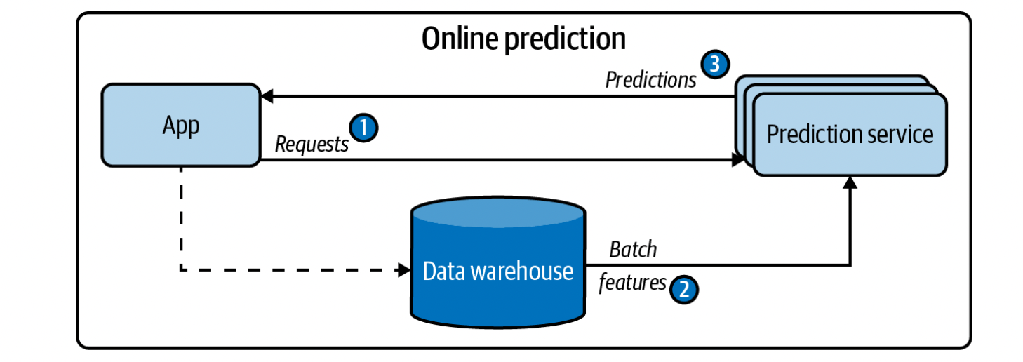
Batch prediction is when predictions are generated periodically or whenever triggered. The predictions are stored somewhere, such as in SQL tables or an in-memory database, and retrieved as needed. This is an asynchronous prediction, since predictions are generated asynchronously from requests. When we do batch predictions, we only use batch features, ie features computed from historical data in a database or datalake. An example is the mean time it takes for an average to make an order.

It’s important to remember that while online predictions aren’t as efficient as batch predictions (since we can’t take advantage of vectorization and parallelization), online predictions often generate less predictions than batching does. The main drawback of batch predictions is that our model is less responsive to a change in a user’s behavior.

The main challenge of online prediction is reducing the latency (end-to-end) to an acceptable level for the user/use-case. There are two things that aid with this:

• A (near) real-time pipeline that can work with incoming data, extract streaming features (if needed), input them into a model, and return a prediction in near real time.
• A model that can generate speed at an acceptable latency for our end-user.

Unifying Batch Pipeline and Streaming Pipeline

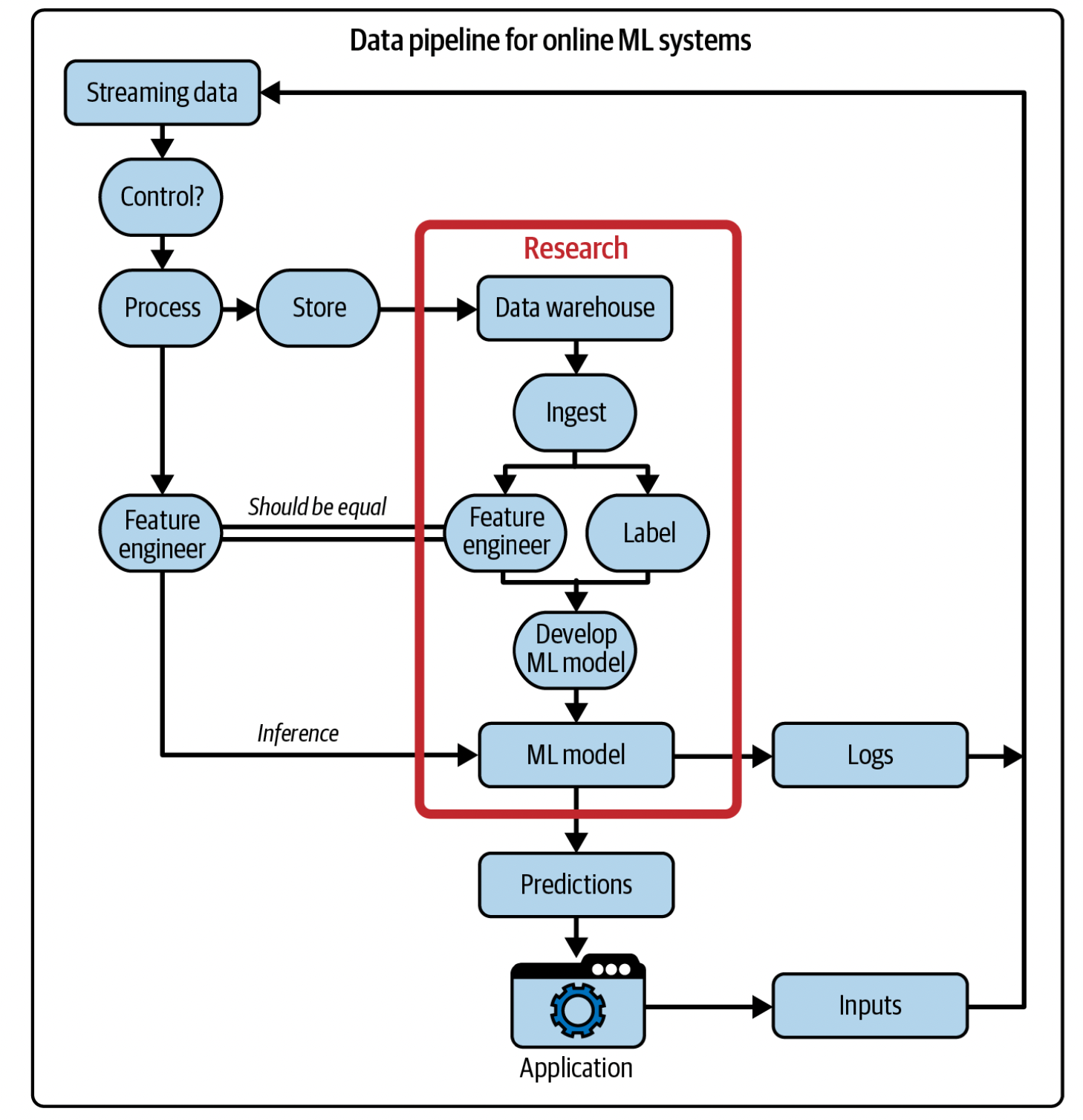
Companies can often benefit from using both batch and streaming predictions to “enhance” their ML models. An example of this is Google Maps. When we compute arrival time, we might train on data from the past month, but during inference we might want to use other information like the average speed of the cars in the past 5 mins.

ML on the Cloud and on the Edge

Deciding if we want our ML applications to run on the cloud or the edge is an important decision to make. Running ML on the cloud is extremely expensive, especially with solutions from AWS/GCP/etc. It also requires an active internet connection, so if network latency is an issue this won’t work. Lastly, edge deployment is better for privacy, since packets aren’t being sent over a network that could be intercepted. The obvious downside of edge computing is the limitation of the chips themselves, regarding memory and computational load, as well as maintaining the battery life.

Detecting Data Distribution Shift

The biggest indicator is if a metric start’s decreasing, accuracy, F1 score, recall, etc. This is generally only possible if our data has “natural” labels.

We can use statistical methods to detect domain shift, comparing min, median, mean, max, percentile (25th, 50th, etc), skewness, kurtosis, etc. We treat our training set as a baseline, and incoming data as our new distribution. We might treat incoming data time series, and measure every data distribution at hour, daily, etc against our baseline.

Monitoring refers to the act of tracking, measuring, and logging different metrics that can help us determine when something goes wrong. We can measure click-rate very easily. We can also use additional metrics, such as watch-time, completion percentage and even a manual report/feedback button to gather more data on our predictions. We can measure our prediction distribution, and assuming that our model hasn’t changed, than different output distributions over time mean a change in inputs over time. We might want to validate that our input features are within an acceptable range (ie age can’t be negative) or if our feature belongs to a pre-determined set.

Observability means setting up our system in a way that gives us visibility into our system to help us investigate what went wrong.

Continual Learning and Test in Production

Most continual learning is not learning on every new sample that comes in. In the case of NNs, this would cause catostrophic forgetting. It’s also not very efficient, since modern systems are optimized for batching. Instead, we update using micro-batches.

We don’t deploy a model until we’ve thoroughly tested it. We create a separate challenger model, to compare its performance to the current champion model in production.

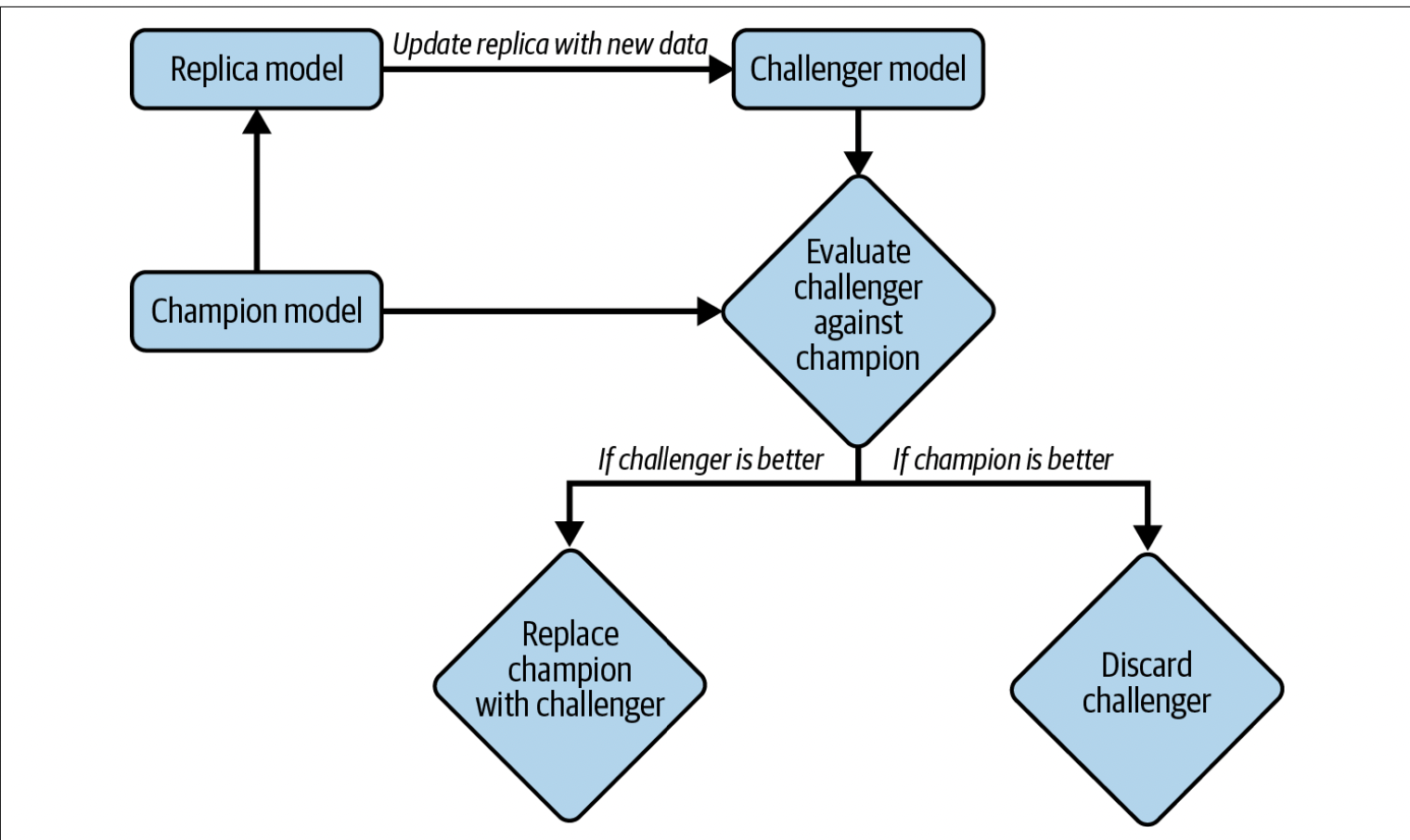
There are two kinds of re-training, stateless training, where the model is retrained from scratch or stateful training, where the model is fine-tuned.

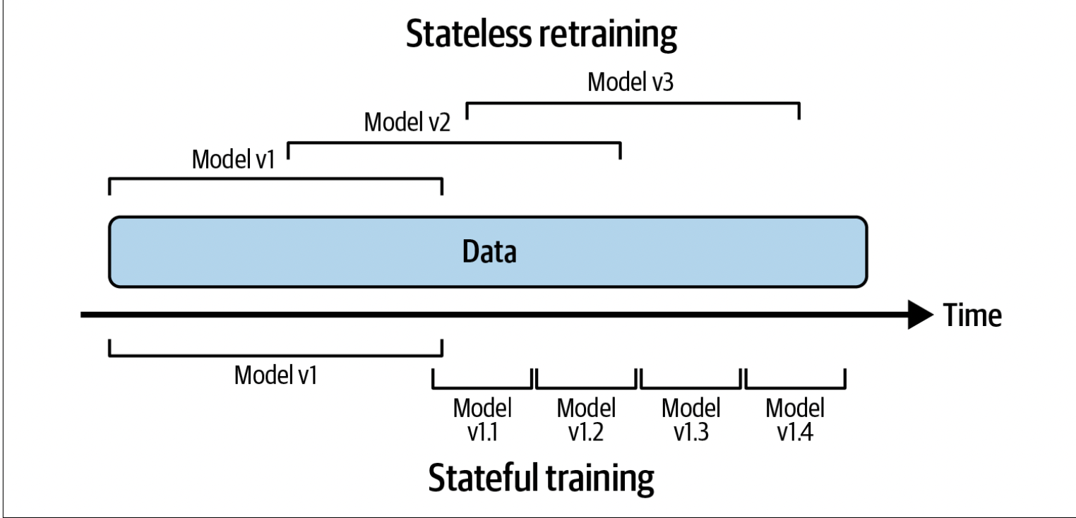
The obvious benefit of stateful training is that we can update our model with less data, while converging faster with less compute required. Another benefit of stateful training is that we don’t need to store the data, which is great if we’re dealing with confidential data. It is common for companies to employ both stateful and stateless training.

The benefit of continous learning is that it allows us to adjust our models to distribution shifts extremely quickly. If we’re uber, and there’s a sudden surge in ride activity in an area that is generally quiet, we want our model to be able to adjust quickly by raising rates.

Continual Learning Challenges

A large bottleneck of continual learning is labeled data. Our models can only be updated when we have the labels to re-train our model. We need to first pull our data from somewhere (most commonly a datalake or from a real time transport service such as Kafka).

The largest challenge is evaluating models, since continual learning amplifies the risk of a catastrophic failure. Each iteration of the model poses another opportunity for it to fail.

Another point of pain are dealing with certain algorithms. NNs work well with fine-tuning with small micro-batches, but matrix based models (like collobrative filtering) and tree-based work quite a bit worse when dealing with this. When dealing with incoming data, if we’re normalizing or using anything that relies on mean, median, etc, it makes it much more difficult to clean our data since we only have access to a subset of our data.

Four Stages of Continual Learning

Testing In Production

Testing offline involves two kinds of testing: test splits and backtesting. Test split act as a static offline method of testing, but are subject to degredation when the split isn’t from the same distribution as the new data. Backtesting is the process of testing a model on data from a specific period of time in the past. Offline evaluation is generally not good enough for continual learning.

A/B Testing

A/B testing is a way to compare two variants of an object, typically by testing responses to these two variants, and determining which of the two variants is more effective.

• Deploy the candidate model alongside the existing model.
• A percentage of traffic is routed to the new model for predictions; the rest is routed to the existing model for predictions. It’s common for both variants to serve prediction traffic at the same time. However, there are cases where one model’s predictions might affect another model’s predictions—e.g., in ride sharing’s dynamic pricing, a model’s predicted prices might influence the number of available drivers and riders, which, in turn, influence the other model’s predictions. In those cases, you might have to run your variants alternatively, e.g., serve model A one day and then serve model B the next day.
• Monitor and analyze the predictions and user feedback, if any, from both models to determine whether the difference in the two models’ performance is statistically significant.

We need to make sure that A/B testing is truly random, or else we’ll be dealing with confounding factors. Secondly, we need to make sure that we run our predictions on a sufficiently large amount of samples to get a holistic view.

Canary Release

Canary release is a technique to reduce the risk of introducing a new software version in production by slowly rolling out the change to a small subset of users before rolling it out to the entire infrastructure and making it available to everybody.

• Deploy the candidate model alongside the existing model. The candidate model is called the canary.
• A portion of the traffic is routed to the candidate model.
• If its performance is satisfactory, increase the traffic to the candidate model. If not, abort the canary and route all the traffic back to the existing model.
• Stop when either the canary serves all the traffic (the candidate model has replaced the existing model) or when the canary is aborted.

The key difference from A/B testing is that we don’t roll out our releases randomly, we might start with a smaller market first.

Interleaving Experiments

Interleaving experiments is the process of displaying both model’s recommendations (for a rec system) to an end user, and seeing which one the users prefer. When applying this to ranking, we know that the top result will always be clicked the most, so we can randomly assign recommendation positions to either model with equal probability.

Infrastructure and Tooling for MLOps

Infrastructure helps automate processes, reducing the need for specialized knowledge and engineering time. Having more mature infrastructure is necessary when we scale our ML applications and data usage.

In the ML world, infrastructure is the set of fundamental facilities that support the development and maintenance of ML systems. There are 4 major systems:

• Storage and compute: The storage layer is where data is collected and stored. The compute layer provides the compute needed to run your ML workloads such as training a model, computing features, generating features, etc.
• Resource management comprises tools to schedule and orchestrate your workloads to make the most out of your available compute resources. Examples of tools in this category include Airflow, Kubeflow, and Metaflow.
• ML platform: This provides tools to aid the development of ML applications such as model stores, feature stores, and monitoring tools. Examples of tools in this category include SageMaker and MLflow.
• Development environment: This is usually referred to as the dev environment; it is where code is written and experiments are run. Code needs to be versioned and tested. Experiments need to be tracked.

Storage and Compute

The storage layer has seen a massive shift to the cloud in the past decade or so. Since storage is cheap, we can use something simple like S3. Next we move onto compute, which we can either use something simple like EC2, or Lambda if our business requirements allow us to go serverless. The benefit of using the cloud is two-fold, one it’s easily scalable up or down as our needs change, and two it takes away alot of developer hours setting up all the infrastucture required.

Resource Management

A cron job allows us to schedule repetitive jobs that run at fixed times. Schedulers are cron jobs that can handle dependencies: ie if job A suceeds, run job B, else run job C. Schedulers deal with job-type abstractions such as DAGs, priority queues, user-level quotas (i.e., the maximum number of instances a user can use at a given time), etc.

ML Platform

While the definition varies from company to company, alot of ML platforming is to provide shared infrastructure across ML applications.

A model store allows us to store our models and their associated meta-data/artifacts. Things we want to keep track of are:

• Model definition: information required to re-create the shape of the model (ie layers of a NN).
• Model parameters: actual values of the parameters of the model. Combined with the definition to get the model.
• Featurize and predict functions: Given a prediction request, how do we extract features and input extracted features to get back our prediction? These are generally wrapped in endpoints.
• Dependencies: eg python version.
• Data: Way of identifying what data was used for training (ie dataset name/version).
• Model Generation Code: this is the code that specifies how are model was created including:
  • What frameworks it used
  • How it was trained
  • The details on how the train/valid/test splits were created
  • The number of experiments run
  • The range of hyperparameters considered
  • The actual set of hyperparameters that final model used
• Experiment artifacts: artifacts generated during training such as the loss curve
• Tags: Tags to aid in discovery and filtering, including the owner of the model and the task it was used for.

A feature store is responsible for 3 main things: feature management, feature transformation, and feature consistency.

• Feature Management: This allows a company to store features that can be used across different models. This can be thought of as a feature catalog, where other teams can browse for features that they might find useful for their model/usecase.
• Feature Computation: The feature engineering logic to extract the features from the data. We can either compute the features every time we access the data if it isn’t too expensive, or just store them after computing them once.
• Feature Consistency: Unify the logic for batch and streaming features to ensure consistency between features during training and during inference. This is because production code might be written in a different language than development code for efficiency reasons.