Adversarial Machine Learning
Some notes I took from learning about adversarial machine learning.
Adversarial Machine Learning
Adversarial machine learning can be loosely defined as a method where we try to fool a model’s output by deceptively modifying the input.
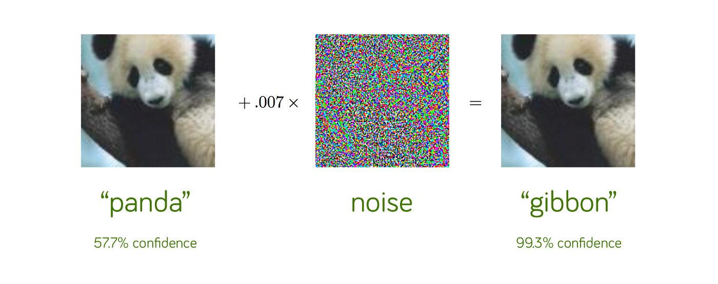
An example of this is a noise attack, where we add some small amount of noise, that is inperceptible to humans, but changes the prediction made by our model.

We have targeted and untargeted attacks.
- Targeted attacks are when we want to trick our model into predicting a certain $y$ output from a given $x$ input. Given an input $x_1$ and its corresponding label $y_1$, we perform a mapping $x_1 \mapsto y_2$, where $y_2$ is a specific output that we’re trying to trick our model to predicting given input $x_1$.
- Untargeted attacks are when we want our model to predict anything but the correct label.
Black Box
Black box attacks occur when adversaries don’t have any access to the model except for its given inputs and corresponding outputs.
White Box
White box attacks are when adversaries have access to the model parameters.
Fast Gradient Sign Method (FGSM) $\to$ We add a certain amount of noise to an image in order to misclasify it. We calculate this as
$adv_x = x + \epsilon * sgn(\Delta_xL(x,y,\theta))$
We calculate our adversarial example $adv_x$ by taking the original input image $x$ and our constant $\epsilon$ which measures our perturbations of our input image, and we take a step in the direction of our gradient $\Delta_x$ with respect to our loss function $L(x,y,\theta)$, ($\theta$ = model parameters and $y$ is the corresponding label to input $x$).
This makes sense intuitively, since we use some form of SGD (like adam) to optimize our NN’s parameters, where we compute gradients and take a step in the opposite direction in order to find the local minima and minimize our loss function. FGSM is essentially perform gradient ascent, where we want to find the local minima with respect to our loss function, in order to miscalculate our predictions.
Deep learning models resistant to Adversarial Attacks
Towards Deep learning models resistant to Adversarial Attacks(Madry et al. 2017)
We can formulize adversarial robustness naively using empircal risk minimization as
$E_{(x,y)\sim D}[L(x,y, \theta)]$
The goal of ERM is to minimize the expected loss of samples drawn from distibution $D$. When we use an attack model, defined by the paper as for each data point $x$, we allow perturbations $S \subseteq \mathbb{R}^d$. This is formulized as
$\underset{\theta}{\min}p(\theta), \;\; where \;\;\; p(\theta) = E_{(x,y)\sim D}\Big[\underset{\delta\in S}{\max}L(x + \delta,y, \theta)\Big]$
Essentially what we’re saying is here that we want to optimize our parameters $\theta$ when given an $x$ and $y$ from distribution $D$ that has been perturbed some $\delta$ amount. This paper then goes onto tackle tackling this saddle point problem as a composition of an inner maximization problem and an outer minimization problem.
- inner maximization: find an adversarial example of a given example $x$ that achieves a high loss i.e. the problem of attacking a given NN
- outer minimization: find model parameters $\theta$ such that when given an adversarial example from an inner attack, we have a minimized loss
The authors state that we can view methods like FGSM and its variations as attempts to solve the inner maximization problem of finding high loss examples with minimal perturbations. On the defense side, we used the perturbed images generated by FGSM as training data in order to make our model more robust to adversarial examples.
The authors use Projected Gradient Descent (PGD) for generating adversarial examples.
$x^{t+1} = \Pi_{x+S}(x^t+\alpha $sgn$(\nabla_x L(x,y,\theta)))$
While the global maxima may be an intractable problem, finding the local maxima isn’t, and local maxima are generally of the same quality. This is empirically the same as finding local minimas when optimizing a NN, where it doesn’t really matter which local minima your model finds.
They find that local maximas found by PGD have relatively the same loss between adversarially trained and non-adversarially trained networks. They also found that if you train your model to be robust against PGD, then your network will be robust against all first-order methods (methods that only require the 1st gradient).
Training adversarially in theory, should generate a more robust model, because for a fixed $S$ perturbations, our decision boundary is much more difficult to model, so successfully doing so should increase robustness.

After training the models (CNNs) on MNIST (convolution with 2 filters -> hidden layer with 64 units -> conv w/ 4 filters with 2x2 max-pooling layers after each convultion.) and CIFAR10 (resnet variation with standard data augmentation and wider layers by a factor of 10). MNIST trained on adversarial examples with $\epsilon = .3$ and CIFAR with $\epsilon = 8$.
$\;\;$Here’s what they find
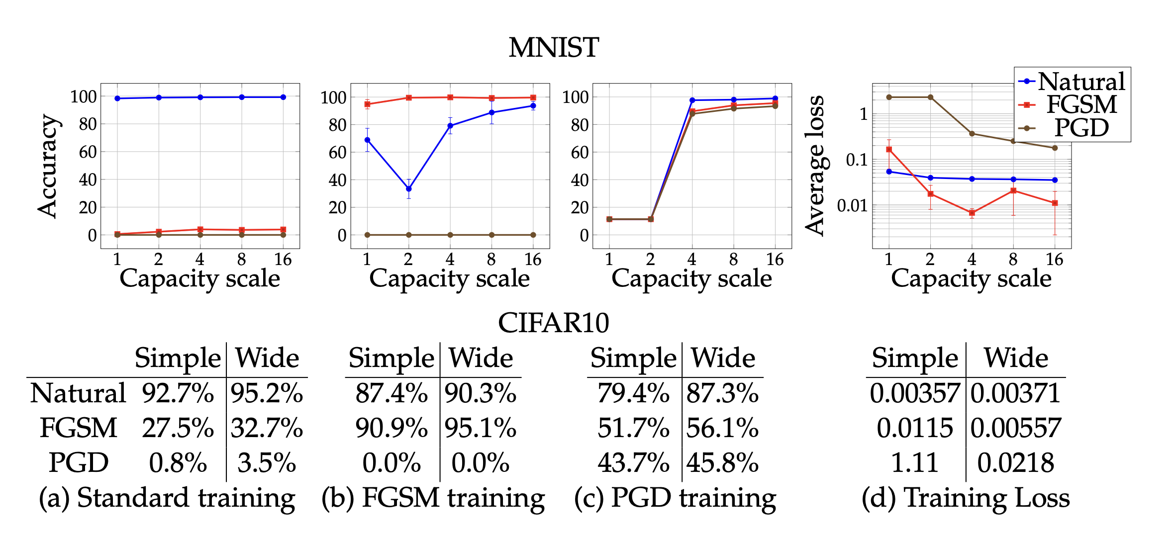
- Capacity alone helps. Scaling the training of only natural examples helps a bit with robustness against one-step perturbations.
- FGSM adversaries don’t increase robustness (for large $\epsilon$). When we train with adversarial examples generated by FGSM, our model overfits, and performs poorly on natural and adversarial examples generated by PGD. When we have small $\epsilon$, our loss is often linear, and adversarial examples generated by FGSM are similar to that PGD, and are suitable for to use to train against PGD.
- Weak models may fail to learn non-trivial classifiers. Small models that would be able to perform well on natural examples end up sacraficing this performance when training with PGD examples, in order to provide robustness against PGD inputs.
- The value of the saddle point problem decreases as we increase the capacity. As we increase the capacity of the model, we can perform better against adversarial examples.
- More capacity and stronger adversaries decrease transferability. Increasing the capacity of the network or using a stronger method for the inner optimization problem reduces the effectiveness of transferred adversarial inputs.
Experiments
As the authors experimented, they focused on a) training a sufficiently high capacity network and b) using the strongest possible adversary. Adversaries were generated using PGD from a random perturbation around the natural input.

We can see from the charts that training with natural or with only FGSM doesn’t lead to adversarial robustness, but when we scale the size of the network, and when we train with PGD, we build robustness with both FGSM adversaries and PGD (as well as natural).